Table Of Contents
What Is XMATCH Function In Google Sheets?
XMATCH is a Google Sheet function that enables users to perform more advanced and customized lookups within their spreadsheets. It works similarly to the popular VLOOKUP and HLOOKUP functions but offers unique features. XMATCH can perform exact matches, approximate matches, and search through sorted or unsorted data arrays. This flexibility allows professionals to easily locate specific values in a large dataset based on specified criteria.
The XMATCH function gives a value from another column corresponding to a specific lookup value.
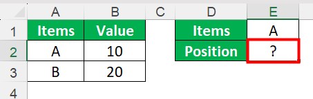
To better understand this concept, let's consider an example where we must find the index value. To achieve this, we can utilize the following formula:
=XMATCH(E1,A2:A3)
The result is shown below.
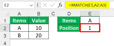
Table of Contents
- XMATCH function in google sheets offers significant improvements over its predecessor, INDEX MATCH.
- The XMATCH is incredibly versatile in handling various scenarios efficiently. Unlike its predecessor MATCH function, XMATCH supports both vertical and horizontal lookups without requiring any transposition of data.
- The XMATCH functionality, like approximate matching with ultimate precision and locale-specific sorting order recognition for non-English alphabets. To sum up, XMATCH provides users with a comprehensive set of syntax and arguments for seamless data retrieval and analysis while maintaining simplicity and precision.
Syntax
=XMATCH (lookup_value, lookup_array, , )
The XMATCH function is designed to search for a lookup value within a lookup array.
By default, it starts searching from the first cell in the array unless otherwise specified. It is important to note that XMATCH only works with a single row or column. In the case of a single row, the first cell would be the leftmost cell, while in the case of a single column, it would be the topmost cell.
When using XMATCH, the match type parameter determines the type of match that Google Sheets will return. A match type of 0 indicates that Google Sheets will only return exact matches. On the other hand, a match type of -1 will return the position of the first entry within the array that is less than or equal to the lookup value. Similarly, a match type of 1 will return the first entry position within the array greater than the lookup value. Lastly, a match type of 2 allows for partial matches, where unknown characters are represented by '?' and unknown strings are represented by '*.'
A search type -1 instructs Google Sheets to search the array in reverse order.
How To Use XMATCH Function In Google Sheets? (With Steps)
To utilize the XMATCH function in Google Sheets, follow these steps.
- First, open our Google Sheet workbook and select the cell where we want the result to appear.
- Next, enter "=XMATCH(" into the selected cell, then specify the lookup value within parentheses. This can be a specific value or a cell reference containing the desired lookup data.
- After that, specify the lookup array using either a range reference or an array constant within parentheses.
- Ensure that the target data for comparison is arranged in ascending order.
- Afterwards, add a comma and specify match mode with an integer parameter between 0 and 3 to define different matching modes (exact or approximate match).
- Lastly, close the formula with a closing parenthesis and press Enter to obtain the result based on specified criteria.
Examples
Example #1 - INDEX And XMATCH
The XMATCH function can be utilized with the INDEX function to retrieve a value from another column corresponding to the lookup value, much like the INDEX MATCH formula.
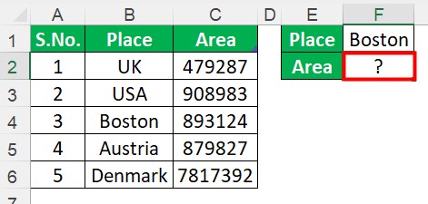
By employing the XMATCH function, the relative position of the lookup value within the lookup array is determined and subsequently passed to the row_num argument of the INDEX function. The INDEX function can retrieve a value from any specified column based on this row number.
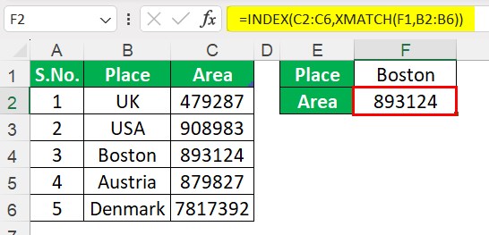
To illustrate, let's consider the scenario where we want to find the area of the place in cell F1. To accomplish this, we can employ the following formula:
=INDEX(C2:C6,XMATCH(F1,B2:B6))
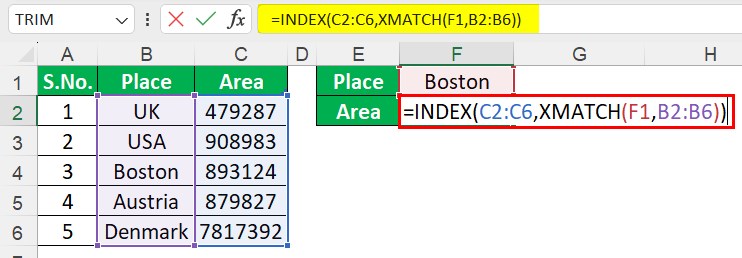
The result is shown in the following image.
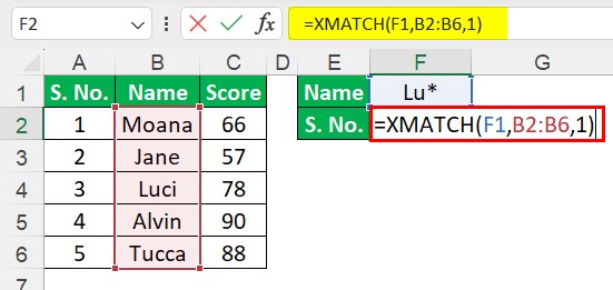
Example #2 - XMATCH With Wildcard
The XMATCH function offers a unique match mode specifically designed for wildcards, which can be activated by setting the match_mode argument to 2.
When utilizing the wildcard match mode, an XMATCH formula allows the use of the following wildcard characters:
- The question mark (?) to match any single character.
- The asterisk (*) to match any sequence of characters.
It is important to note that wildcards only apply to text and cannot be used with numbers.
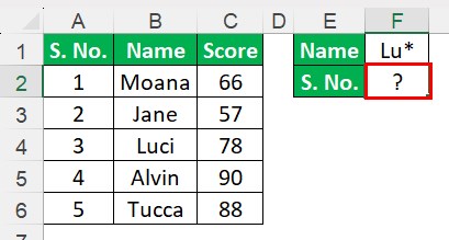
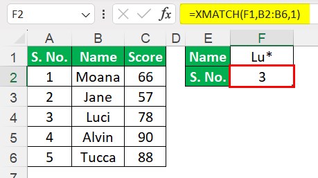
To illustrate, let's consider an example where we want to determine the position of the first item that begins with "Lu*." In this case, the formula to be used is:
=XMATCH(F1,B2:B6,1)
The result is shown in the following image.
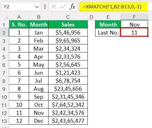
Example #3 - XMATCH Reverse Search
In situations where the lookup value appears multiple times in the lookup array, it may be necessary to determine the position of the last occurrence.
The direction of the search is determined by the fourth argument of XMATCH, known as search_mode. To conduct a reverse search from bottom to top in a vertical array and from right to left in a horizontal array, the search_mode should be set to -1.
To illustrate this, let's consider an example where we want to find the position of the last record for a specific salesperson.
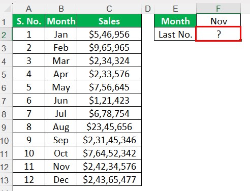
By combining the four arguments, we can construct the following formula:
=XMATCH(F1,B2:B13,0,-1)
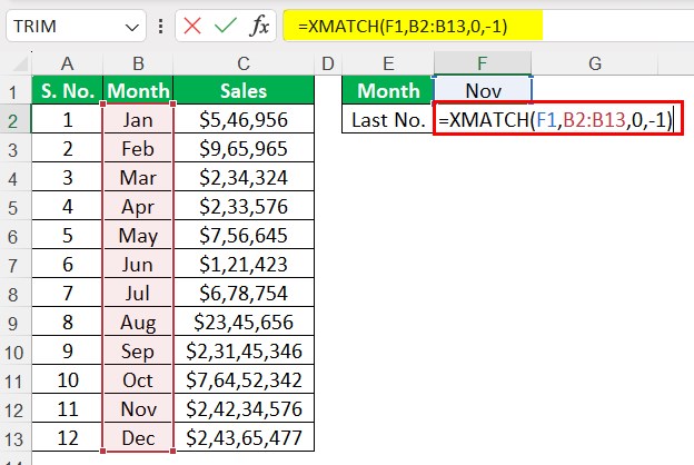
This formula will give us the number corresponding to the last sale made in Nov.
Example #4 - Compare Two Columns For Match
To compare two lists for matches, we can utilize the XMATCH function in conjunction with IF and ISNA. This powerful combination allows us to identify matches between the lists efficiently.
For example, we want to compare List 2, located in cells B2 to 7, against List 1 in cells A2 to A7.
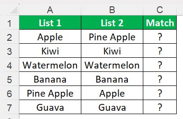
To achieve this, we can use the following formula:
=IF(ISNA(XMATCH(B2:B7,A2:A7)),"","Match Found")
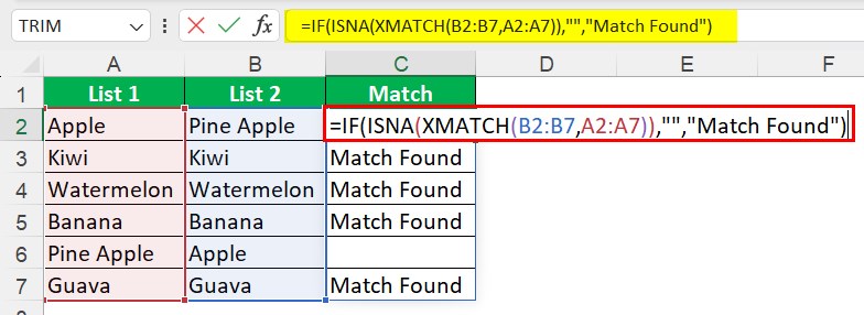
The result is shown in the following image.
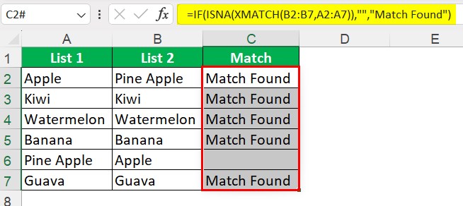
In this particular scenario, we are solely interested in identifying matches. Therefore, the value_if_true argument of the IF function is an empty string denoted by (). This ensures that only the matches are displayed.
Important Things To Note
- The XMATCH function can handle horizontal and vertical searches, making it highly versatile.
- This feature is its ability to find the relative position of a lookup value within an array, which can be useful for financial modeling or data analysis purposes.
- It enhances efficiency by eliminating the need for complex nested formulas or unnecessary data sorting before conducting searches.
- XMATCH function helps professionals save time and effort when working with complex datasets in Google Sheets.
Frequently Asked Questions (FAQs)
● Firstly, XMATCH only supports single-dimensional arrays, which means it cannot be used with multi-column or multi-row data ranges.
● Additionally, the XMATCH function cannot perform approximate matches or handle wildcard characters like "*" or "?". It also lacks a binary search option and cannot handle certain data formats like dates or text.
● Another limitation is that XMATCH is only available in versions of Google Sheets that support dynamic array formulas.
● Therefore, if we work with an older version of Google Sheets, we won't be able to take advantage of this function.
Despite these limitations, the XMATCH function remains a powerful tool for performing exact match lookups within single-dimensional data sets incompatible versions of Google Sheets.
The XMATCH function, introduced in Microsoft Google Sheets 365, offers valuable functionality in various scenarios. One common use case is in data analysis involving multiple criteria matching.
Another practical application is data cleansing and validation. When duplicates or errors are present within a dataset, XMATCH can swiftly identify these instances and aid their resolution.
Similarly, when working with time-sensitive data, such as stock prices or temperature readings over a particular period, XMATCH enables users to find the closest match for a given date or timestamp within the dataset.
The XMATCH function, introduced in Google Sheets 2021, is a powerful tool for advanced data lookup capabilities. Its syntax is straightforward and consists of three main arguments. The first argument represents the lookup value we wish to find within a specified array or range. The second argument signifies the array or range where we want to perform the lookup. An optional third argument allows us to define the match type, using "0" for an exact match, "-1" for the closest smaller value, or "1" for the closest larger value.
The XMATCH function retrieves a value from another column corresponding to a specific lookup value.
To better understand this concept, let's consider a scenario where we need to find the index value. To accomplish this, we can make use of the following formula:
=XMATCH(F1, A2:A3)
The resulting value is displayed below.
Download Template
This article must help understand the XMATCH function Google Sheet examples. You can download the template here to use it instantly.
Recommended Articles
This has been a guide to What Is XMATCH Function In Google Sheets. We explain the How To Use XMATCH Function In Google Sheets with examples. You may learn more from the following articles –
