XLOOKUP

Last Updated :

21 Aug, 2024

Blog Author :

Edited by :

Reviewed by :

Table Of Contents

XLOOKUP Function Definition

The XLOOKUP Excel function finds specific values in an array range vertically or horizontally, with an approximate, exact, or partial match. The advantage of XLOOKUP is that it allows you to search for results both to the left and right of your search value in rows and columns. However, it is a new function available only from 2020 for Excel users.

For example, in the below table, you can look up a student’s marks using their roll. Enter the formula in cell F3 as =XLOOKUP(E3,A2:A6,C2:C6). You get 49, the marks secured by the student with roll number 1003.

XLOOKUP Function Definition

The XLOOKUP function can perform complex searches with multiple criteria. In addition, it can perform both horizontal and vertical searches.
We can use it to return an entire row or column, not just a value. We can also use it with wildcard characters for partial searches.
You can print an alternate message if the lookup value does not find a match.
It can be used as an alternative to the HLOOKUP and VLOOKUP functions since it is more versatile. For example, you can find an exact, approximate, or partial match.

XLOOKUP Function

The syntax of the XLOOKUP function is as follows:

Arguments

lookup_value - (mandatory)The lookup value we will retrieve the result from the array specified in return_array.
lookup_array - (mandatory) The array or range of cells searched
return_array - (mandatory) The array or range of cells from which the value is returned
- (optional) The text value to be printed if it does not find a match in the return_array. If this argument is blank, you get a #N/A error if there is no match.
- (optional) It specifies the type of match. The values are:

0	It is the default value. It searches for the exact match specified in *lookup_value*. If there is no match, it returns a #N/A error unless you mention the argument.
-1	Searches for an exact match. If not found, returns the next smaller value.
1	Searches for an exact match. If not found, it returns the next larger value.
2	Performs a wildcard match with the characters *, ?, and ~.

– (optional) Here, we specify how to search. The values are:

1	It is the default value. Here, the search is done from the first item to the last in the lookup_array.
-1	The search is done in reverse, from the bottom to the top.
2	It performs binary searches on the array sorted in ascending order. If not sorted, you will get an error.
-2	It performs a binary search on data sorted in descending order. It will also throw an error if unsorted.

How To Use XLOOKUP

The XLOOKUP function is an improved version of the VLOOKUP. Here, it can search a range of cells instead of a column. In addition, we can manually enter the function in any cell or through the Excel ribbon.

1. Entering XLOOKUP In Excel Manually

Below is an Excel sheet containing the names of all eight planets in the solar system and their total number of moons.

XLOOKUP Excel Function - Entering XLOOKUP in Excel manually

In this example, let us find the number of moons of Saturn.

We must look up any planet and check its number of moons. For this, use the planet name as the lookup value, the lookup range(B2:B9), and the return array(C2:C9) as arguments.

Enter the formula in cell F3. Here, the first argument is the reference of the lookup value.
Next, select the lookup range. In this case, it will be the planets in Column B. Select the cells from B2 to B9.
The third argument is the return array in Column B containing the number of moons. Select the cells from C2 to C9.
Now, close the bracket and press Enter. You get the number of moons of Saturn in cell F3, which is 83. Note that we have not specified the other optional arguments as we perform a simple search and retrieval.

Thus, the function is simple and easy to use when entered manually.

2. Entering XLOOKUP in Excel through the Excel Ribbon

The XLOOKUP shortcut method is to enter it through the Excel ribbon. Then, place the cursor in the cell where you need to insert the formula.

To obtain the XLOOKUP shortcut, go to the Excel ribbon and click on the Formulas tab.
Under the “Functions Library,” select “Lookup & Reference.” Choose the XLOOKUP option.

XLOOKUP Excel Function - Entering XLOOKUP in Excel through excel ribbon

You will get a pop-up window where you can enter the arguments.

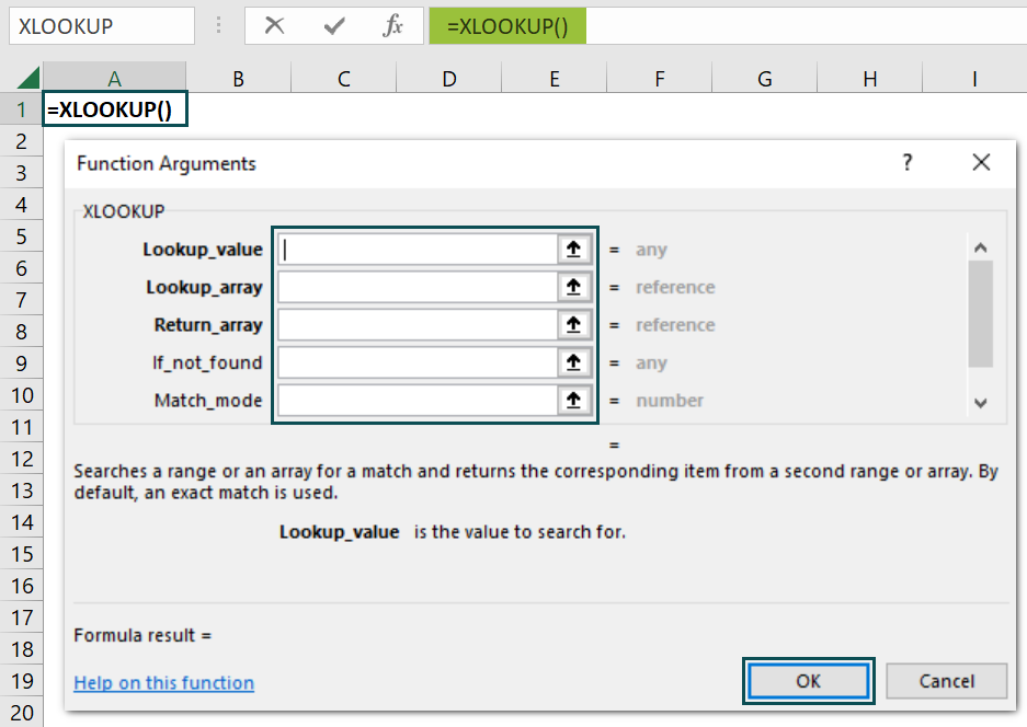
XLOOKUP Excel Function - Functions arguments window

The XLOOKUP function can be used in multiple ways, as seen in the examples below.

Examples

XLOOKUP() can replace the VLOOKUP function with its versatility and ease of use. The examples below show us how to use the function to look up specific values in a range.

Example #1

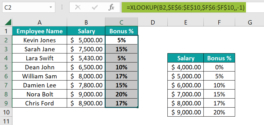
Let us look at how the function does an approximate match. In the XLOOKUP example below, we have some employees' Employee Name (Column A) and Salary (Column B) details. Based on their salary, ), their Bonus % ( Column C) is determined. The range E4:F10 contains the bonus details for different salary brackets.

Step 1:
- Employees earning between $ 4,000 to $ 5,000 would get a 0% bonus. Those earning between $ 5,000 to $ 6,000 would get a 5% bonus, and so on.
- To find an approximate match, we must enter the fifth argument as -1. Then, it searches for the specified value, and if there is no match, it returns the next smaller value.
- Suppose an employee earns $ 5,500; it would find and match $ 5,000, the next lower value, and return its corresponding bonus, 5%.

Enter the formula =XLOOKUP(B2,$E$5:$E$10,$F$5:$F$10,,-1) in cell C2 and press Enter. Note that we have not specified any value as the fourth argument. We add “$” to these two arrays to make them absolute references, as their values must not change.

Step 2: Drag the Autofill handle from C2 to C9 to get the bonus % for all the employees.

Example #2

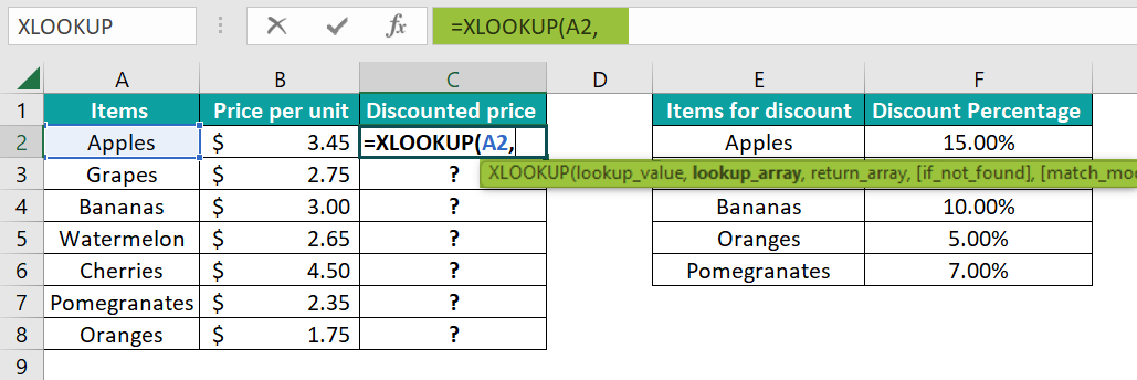
Below is a table containing the names of some items at a supermarket and their unit price. The supermarket offers discounts on some of its items listed in Columns E and F.

Columns B and F have been formatted as Currency and Percentage, respectively. Next, we must apply the discount percentage to the items in Column A and calculate their discounted price.

Step 1: We are looking for a discount on the first item, Apple. Enter the formula in cell C2.

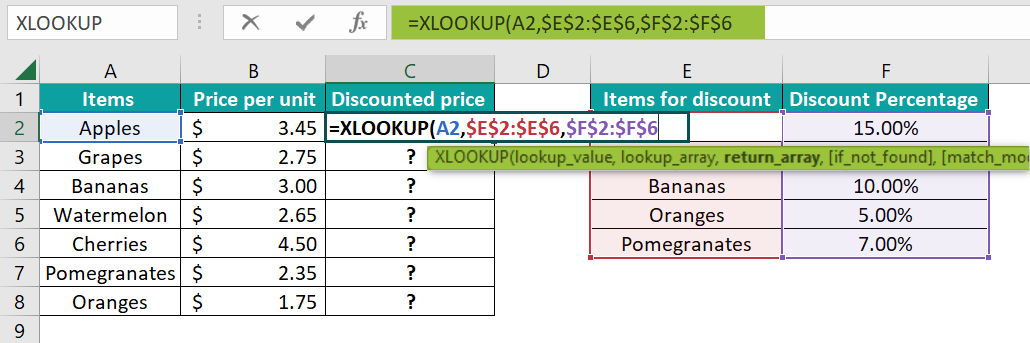
Step 2: Column E contains the item names, and Column F, the discount percentage.

Select cells E2 to E6 and F2 to F6 as the lookup_array and return_array, respectively. Here, we add “$” to these two arrays to make them absolute references.

Step 3: Now, we need the discounted price in Column C
- Multiply the output of the function by the price per unit (B2)
- Subtract it from the initial price B2 to get the discounted price.

Applying the above changes, we enter the formula in cell C2 as

=(B2 - (XLOOKUP(A2,$E$2:$E$6,$F$2:$F$6)*B2)).

Drag the Autofill handle from C2 to C8 to get the discounted prices of each item.

Step 4: You must have noticed the #N/A error. It appears for items that do not have a discount specified in Columns E and F. To avoid this error, we can supply the fourth argument to the formula as 0.

Step 5: Press Enter. Drag the Autofill handle from C2 to C8 to get the discounted price of each item.

Also, since we supplied zero as the fourth argument, the items not found on the discount list have the same price after the discount.

Example #3

We can perform an XLOOKUP two-way lookup by nesting one XLOOKUP function within another. Here, the inner function returns a result that the outer function will use.

Below is an XLOOKUP example of a few students’ names and marks in Physics and Chemistry. Here, we can find the values of a student’s marks in either Physics or Chemistry by entering the details in cells F3 and F4.

Step 1: Here, we enter a formula in cell F5 to find the marks of student “Susan” in Physics as follows:

=XLOOKUP(F4, B1:C1, XLOOKUP(F3, A2:A7, B2:C7)

Step 2: Press Enter. You get the result as 76, the mark secured by the student “Susan” in Physics.

Explanation:

The formula =XLOOKUP(F4, B1:C1, XLOOKUP(F3, A2:A7, B2:C7) has a nested function.

The inner XLOOKUP(F3, A2:A7, B2:C7) retrieves the data of “Susan.” Here, F3 is the lookup value, and A2:A7 is the lookup array where it looks for the name “Susan.” The fourth row contains her marks in Physics and Chemistry.
B2:B7 is the array where the data is present.
The function returns the fourth row as an array. So, the output of the inner function is {76,90}.
The outer array looks like =XLOOKUP(F4, B1:C1, {76,90}).
It finds F4(“Physics”) in the lookup range B1:C1. It is the first item in this range, so its corresponding value from the array, 76, is returned.

Important Things To Note

XLOOKUP() allows you to specify a range of cells as the return array instead of just a column index.
It can also look for data to the left of the selected cell. So, column orders do not matter.
XLOOKUP provides an exact match by default. It can also look up data from the bottom to the top.
The XLOOKUP in excel not working criteria happens if it does not find the lookup value and you get an #N/A error.

Frequently Asked Questions (FAQs)

1. Is XLOOKUP better and faster than the VLOOKUP?

Yes, the XLOOKUP function is faster than VLOOKUP and more versatile. Unlike VLOOKUP, it can search both horizontally and vertically. It can also look up values to the left of the search column.

2. Can XLOOKUP Return Multiple Values?

XLOOKUP currently returns a single value or an array with multiple items when it finds a match to the search criteria.

3. What is the difference between HLOOKUP and XLOOKUP?

HLOOKUP
• In HLOOKUP, H stands for “Horizontal.”
• This function performs a horizontal lookup.
• It searches the rows of a table and returns a specified value from a row.
• You must supply the row index number as its third argument.

XLOOKUP
• It looks up both rows and columns and returns a specified value.
• It can return value from a range of cells, not just a column.
• XLOOKUP can look up data from an array on the left side of the lookup value.

4. Can you use XLOOKUP with multiple criteria?

Yes, you can use the function with multiple criteria. For example, you can combine different expressions using Boolean logic when supplying the lookup array argument.

Download Template

This article must help understand the XLOOKUP Excel function’s formula and examples. You can download the template here to use it instantly.

XLOOKUP Download