Wrap Text in Excel

Last Updated :

Blog Author :

Edited by :

Reviewed by :

Table Of Contents

What is Wrap Text in Excel?

The wrap text feature in excel allows displaying lengthy text strings of a cell in multiple lines. This enhances the readability of the worksheet and ensures that the entire cell data is visible at all times. After wrapping text, the row height increases automatically though the column width stays the same. If one changes the column width, the cell content adjusts itself to fit the new width.

For example, in the following image, wrap text has been applied to the string in cell B2. At the same time, column B has been widened.

The purpose of wrapping text is to prevent the cell data from spilling to the cells on the right. Moreover, it ensures that a text string is not cut by the border of the adjacent cell. Wrapping text is extremely helpful in worksheets that have a lot of content to display at a time.

What is Wrap Text in Excel?

How to Wrap the Text in Excel?

Wrap text is a formatting feature of Excel, which changes the appearance of a string without changing the string itself. The methods of wrapping text are listed as follows:

Method #1–Wrap text using the Home tab
Method #2–Wrap text using the “format cells” window
Method #3–Wrap text using the keyboard shortcut
Method #4–Wrap text using line breaks

Note that methods #1 to #3 wrap text automatically, while method #4 wraps text manually. In method #4, line breaks are inserted at the desired place in a cell. A line break serves as a substitute for the wrap text feature of Excel.

Let us discuss the four methods with the help of examples.

Method #1–Using the Home tab

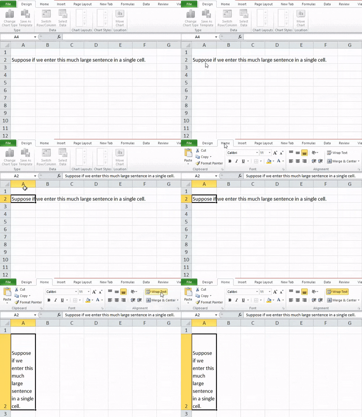
The succeeding image shows a long text string in cell A2. We want to wrap this text in cell A2. Use the “wrap text” option of the Home tab.

The steps to wrap text in excel by using the stated method are listed as follows:

Step 1: Select cell A2 whose text string needs to be wrapped.

Step 2: From the “alignment” group of the Home tab, click “wrap text.” The text string of cell A2 is displayed in multiple lines, as shown in the succeeding image.

Notice that even after wrapping text, the width of column A stays the same as that of the other columns. However, the height of row 2 increases when this feature is turned on.

Note 1: “Wrap text” is a toggle button that can be turned on and off to wrap and unwrap the text.

Note 2: To wrap the text of multiple cells simultaneously, select all such cells and press the “wrap text” toggle button.

Method #2–Using the “Format Cells” Window

Working on the text string of method #1, we want to wrap the text in cell A2. Use the “format cells” window of Excel.

The steps to wrap text in excel by using "Format Cells" are listed as follows:

Select cell A2 containing the string to be wrapped. Right-click the selection and choose “format cells” from the context menu.
Alternatively, press the shortcut “Ctrl+1” after selecting the cell.
The “format cells” window opens, as shown in the following image. Click the “alignment” tab. Then, from “text control,” choose the “wrap text” option and click “Ok.”
The wrap text feature has been applied to cell A2, as shown in the following image. This time also, the width of column A has not changed, but the height of row 2 has increased.

Method #3–Using the Keyboard Shortcut

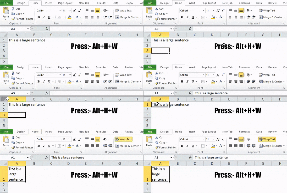
The succeeding image shows a text string in cell A1. We want to wrap this string of cell A1. Use the keyboard shortcut for wrapping text.

The steps to wrap text in excel by using keyboard shortcut are listed as follows:

Step 1: Select cell A1 that consists of the string to be wrapped.

Step 2: Press the shortcut keys “Alt+H+W.” For this shortcut to work, first press the “Alt” key and release it. Next, press and release the “H” key followed by the “W” key.

Step 3: Once the “W” key is released, the “wrap text” feature is applied to the cell selected in step 1. The output is shown in the following image.

Method #4–Using Line Breaks

Working on the text string of method #1, we want to perform the following tasks:

Apply the wrap text feature in cell A1.
Insert line breaks manually after the strings “enter,” “large,” and “a” in cell A2.
Compare the results of applying wrap text with inserting line breaks.

Use the keyboard shortcut for inserting line breaks. Note that both cells A1 and A2 should contain the text string of method #1.

The steps to perform the given tasks are listed as follows:

Step 1: Wrap the text in cell A1 by selecting the cell and choosing “wrap text” from the Home tab. The output is shown in cell A1 of the succeeding image.

Step 2: To insert line breaks, place the cursor in that part of the cell where line breaks are to be inserted. Next, press the keys “Alt+Enter” together.

So, first, place the cursor after the string “enter” and press the given shortcut. The line break is inserted at the end of this string. Likewise, insert line breaks after the strings “large” and “a.”

The result is shown in cell A2 of the following image.

Comparison between applying wrap text and inserting line breaks: It must be noted that when a line break is inserted, the “wrap text” feature is automatically turned on in Excel.

Therefore, when “wrap text” is applied, it is applied alone. However, when a line break is added, it is added in combination with “wrap text.”

The line breaks entered in cell A2 will stay in place even if column A is made wider. Moreover, if “wrap text” is turned off but the line breaks are retained, the string of cell A2 appears in a single line. However, the line breaks inserted in step 2 are visible in the formula bar.

In contrast, when the “wrap text” of cell A1 is disabled, the string appears as a single line, in this cell and the formula bar. So, with wrap text in excel, the cell content can regain its initial appearance with a single click of the toggle button.

The Reasons “Wrap Text” Feature may not Work in Excel

The reasons due to which the wrap text feature may not work in Excel are listed as follows:

It does not work on merged cells. So, cells need to be unmerged before the wrap text feature can be applied to them.
It does not work if the cell is already wide enough to display the entire text string. In this case, one can insert line breaks to display the cell content in multiple lines.
It may not be visible if the height of the row has been set at a very low value. To avoid this, make sure that the height of the row adjusts automatically with the application of the wrap text feature in excel.

Note: To ensure that wrapped text is visible at all times, follow either of the listed techniques in Excel:

Set the row height to adjust automatically. For this, click the “format” drop-down from the “cells” group of the Home tab. Next, choose “AutoFit row height” from the “cell size” option.
Enlarge the height of the row manually. For this, place the cursor on the lower border of the row label. The row labels are displayed on the left side of the worksheet. Once the “resizing” mouse pointer appears, drag the lower border of the row downwards to increase the row height.

Frequently Asked Questions

1. What is the wrap text feature and where is it in Excel?

The wrap text feature in excel helps display the content of a cell in multiple lines. With wrap text, the text is wrapped in such a way that the row height increases, but the column width stays the same. Further, the column width can be increased or decreased by the user. The text string adjusts itself automatically with a change in the column width.

However, even after applying the wrap text feature, one can maintain a consistent column width throughout the worksheet. The “wrap text” is a toggle button of Excel, which is available in the “alignment” group of the Home tab.

Note: For more details on the working of the wrap text feature, refer to the examples of this article.

2. List the reasons and state the shortcut of using the wrap text feature in Excel.

The wrap text feature is used in Excel for the following reasons:

• To prevent text strings from being truncated by the adjacent cell
• To avoid overlapping of text strings
• To ensure that the entire cell content is visible
• To improve the readability of large datasets
• To make the worksheet neat, organized, and fit for printing

In Excel, the shortcut of wrapping text is “Alt+H+W.” All the keys must be pressed one after the other in the given sequence. Prior to using this shortcut, ensure that the cell, whose text is to be wrapped, is selected.

3. How to wrap text without expanding the size of the cell in Excel?

After applying the wrap text feature, one can keep either the row height or the column width constant but not both simultaneously. If both (row height and column width) are held constant, the wrapped text will not be visible.

The steps to keep the row height constant are listed as follows:

• Select the cell in which the text is to be wrapped.
• Click the “format” drop-down from the “cells” group of the Home tab.
• From “cell size,” select “row height.”
• In the “row height” window, do not enter any value. Simply click “Ok.”

Now, when the wrap text feature is applied to the selected cell, the row height will remain the same as that of the other rows. On the other hand, the column width already stays constant even after applying the wrap text feature.

However, when the text of a cell is wrapped, it is recommended that one should not prevent a cell from expanding. This is because the basic purpose of wrap text will not be served if the cell is not permitted to enlarge.