Table Of Contents
What Is Week Number In Excel (WEEKNUM)?
WEEKNUM or Week Number in Excel is a Date & Time function that gives us the week number for the given date. We know that we have an average of 52 weeks in a year for 12 months. So, for a particular date, the Excel Week Number helps us find the specific week number.
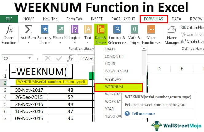
For example, for the dates given below in cells A1:A7, when we apply the WEEKNUM Excel function for the cell B1, and then drag the formula using the fill handle to the rest of the cells, i.e., to cells B1:B7, we will get the output shown below.

Key Takeaways
- The Week Number in Excel helps users retrieve the precise serial number of the week of a specific date out of the approximate 52 weeks per year.
- We use the WEEKNUM function that has two arguments:
- The first which is mandatory takes valid date.
- The second argument is optional, which represents the day on which the week begins.
- The start of the year, Jan 01, will always be the first week of the year, and Dec 31 will always be the last week of the year, the 52nd week.
- We have 10 different options to supply at the start of the week. Since this is an optional argument, we need not mandatorily supply the argument.
- However, if we leave this argument blank, by default, the value will be 1, i.e., the start of the day of the week is Sunday.
Syntax Of WEEKNUM Function In Excel
The syntax of the WEEKNUM formula is,

The arguments of the WEEKNUM formula is,
- serial_number: It is the date for which we find the week number. Excel treats DATE as a serial number.
- return_type: We need to mention the start of the weekday.
How To Use The Week Number (WEEKNUM) Function In Excel?
We can use the WEEKNUM function in Excel as follows:
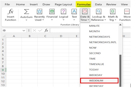
First, choose an empty cell - select the “Formulas” tab - go to the “Function Library” group - click the “Date & Time” option drop-down - select the “WEEKNUM” function, as shown below.

Examples
We will consider some examples to use the WEEKNUM Function in Excel.
Example #1 – Finding Week Number in Excel
We have the below dates and must find the Excel Week Number for each date in that particular year.

The steps to find the Week Number are as follows:
Open the Excel WEEKNUM function in the B2 cell.

The serial_number is nothing but your date cell. So, select A2 as the cell reference.

As of now, ignore the last argument. By default, it will take Sunday as the starting day of the week.

Drag the formula to other cells.

We got week numbers for respective dates. But look at the cells A2 and A3; both are on 30th Nov but of a different year. Since Excel considers the start of the week from Sunday, it will vary year to year.

Now, let us change the start of the week to MONDAY.

We can mention the argument as 2. Close the formula.

The result is shown below:

Apply to other cells by dragging the formula.

We do not see any differences here. Try changing the starting day of the week to a different date and find the differences.
Example #2 – Add the Word WEEK to the Week Number in Excel
We have seen how to return the week number of any supplied date. It will be clearer to add the word “Week” before the week’s number, like in the image below.

It is where the advanced formatting technique in excel comes into the picture. Follow the below steps to apply the above formatting.
- Step 1: Select all the result cells first.

- Step 2: Right-click on the selected cells and select “Format Cells”.

- Step 3: Now, we will see the format dialog box. Go to “Custom” first.

- Step 4: Enter the format code “Week”# in the Type: field.

- Step 5: Press “OK”. We will have results ready.

Instead of changing the formatting of the cells, we can also combine the word “Week” with the result cells. Refer to the image to apply the same.

Example #3 – Calculate Number of Weeks in excel between Two Dates
We have learned the technique of finding the week number. But, how to tell how many weeks are between two dates?
If we have started the project on 15th Jan 2018, and completed it on 30th April 2018, as shown below.

The steps to calculate the weeks taken to complete the project are,
- Step 1: Firstly, find the difference between the two dates.

- Step 2: Now, divide the difference by 7. We have 7 days a week.

- Step 3: Press the “Enter” key to complete the formula. We have a result like this.

- Step 4: Change the format to “General” for accurate results.

Example #4 – Calculate the Number of Weeks in Fraction using Excel
Let us consider one more example to have a clear idea about finding the week’s number between two dates in Excel.
Suppose we are going on a business trip from 15th Feb 2018 and are returning on 30th Jun 2018. The business head decided to pay the money weekly.

Let us apply the formula we used in the previous example to find the difference between the two dates.

Now, divide the difference by 7. So, we have 7 days a week.

We have a result like this.

Let us change the format of the resulting cell to fractions.

So, we have the number of weeks in fractions now.

Important Things To Note
- By default, the start of the week in Excel is SUNDAY.
- We must supply the return type correctly to start with a different week.
- If the date is not in the correct format, we may get #VALUE! error.

