VLOOKUP True

99.99% of the time, everybody uses FALSE as the range lookup criteria because 99.99% of the time, we need an exact match from the table array. Even in the training sessions, your trainers must have explained only FALSE criteria and would have said not to worry about the TRUE criteria. We have not used TRUE criteria because of the not arising scenario. Still, this article will show you how to use TRUE criteria in VLOOKUP with different scenarios.

First, take a look at the syntax of the VLOOKUP formula.

All the arguments of the VLOOKUP function are mandatory in the above syntax, but the last argument is optional. Therefore, we can supply this argument with two parameters: TRUE (1) or FALSE (0).

It will find the approximate match if you supply TRUE (1). It will find the exact match if you supply FALSE (0).

Now, take a look at the below data set in Excel.

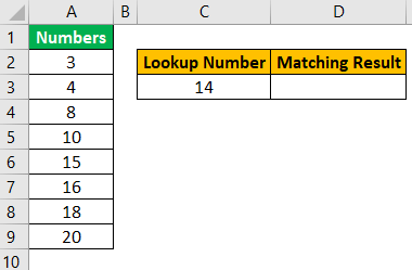
Above, we have numbers from 3 to 20. On the right-hand side, we have a lookup_value of 14, but this number does not exist in the main numbers table.

First, apply the VLOOKUP function with FALSE as the range lookup criteria to find the exact match.

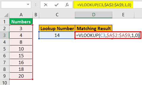
Now, press the "Enter" key to get the result of the formula.

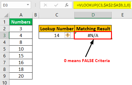
As a result, we have an error value of not available #N/A.

Now, change the range lookup criteria from FALSE (0) to TRUE (1).

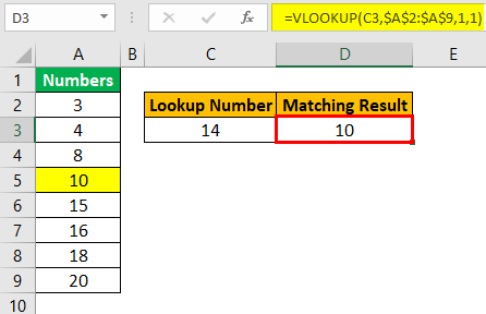
This time we got a result of 10. You must be wondering about the number 14, which does not exist in the table array. How did this parameter return 10 as a result?

Let me explain to you the result for you.

We have set the range lookup argument as TRUE, so it finds the closest match for the lookup value provided (14).

It works because our lookup value is 14, and the VLOOKUP starts to search from top to bottom when the lookup_value is lesser than the value in the table it will stop then return the respective result.

For example, in our data, 14 is greater than 10 and less than 15, so the moment VLOOKUP finds the value 15, it will return and provide the previous smaller value, 10.

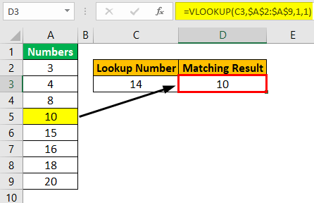
To test this, change the value from 10 to 15 and see the magic.

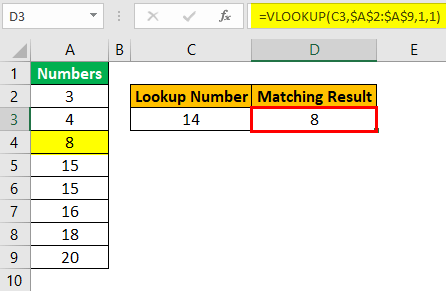
Because we have changed the current lesser value more than the lookup, it has returned the previous lesser value, 8.

IF is an important function in Excel, and we use IF statements for all the criteria-based calculations. For example, look at the below data.

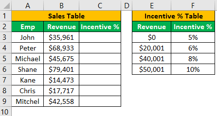
We have two tables: the “Sales Table” and “Incentive %” Table.” For the “Sales Table,” we need to arrive at an "Incentive %" based on the revenue generated by each employee. To calculate "Incentive %," we have the below criteria.

• If the revenue is >50000, then the incentive % will be 10%.
• If the revenue is >40000, then incentive % will be 8%.
• If the revenue is >20000, then incentive % will be 6%.
• If the revenue is <20000, then incentive % will be 5%.

So, we have four criteria to satisfy. In these cases, we use typical IF conditions to arrive at incentive %, but now see how we can use VLOOKUP to reach incentive %.

Apply the VLOOKUP formula with TRUE as the criteria.

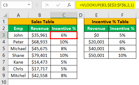
We have our incentive % against the revenue generated by each employee. Let me explain to you how this works.

First, look at the Incentive % table.

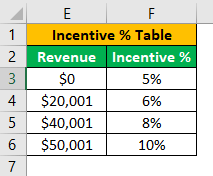
• It says between 0 to 20000 incentive % is 5%.
• Between 20001 to 40000, incentive % is 6%.
• Between 40001 to 50000, incentive % is 8%.
• Anything above 50000 incentive % is 10%.

Since we have provided TRUE as the range lookup argument, it will return the approximate match.

Look at the first case: this revenue is 35,961, less than the incentive table value of 40,000, and less than 40,000 in the table is 20,000. So for this, the "Incentive %" is 6%.

Like this, the TRUE function works and says goodbye to complex IF conditions.

• TRUE finds the approximate match.
• TRUE is also represented by 1.
• In the case of a numerical scenario, it always finds the less than or equal to the lookup value in the table array.
• If the lookup_value is lesser than all the values in the lookup table, it will return an error like #N/A.