VLOOKUP with Multiple Criteria

Sometimes while working with data, when we match the data to the reference VLOOKUP, if it finds the value first, it displays the result and does not look for the next value. But, what if the user wants the second result? It is another criterion. To use VLOOKUP with multiple criteria, we need to use other functions, such as the CHOOSE function.

Let us now see examples of the VLOOKUP function with multiple criteria search.

Suppose you have data of employees of your company. The data contains the "Name," "Current Salary," "Department," and "ID," as shown below.

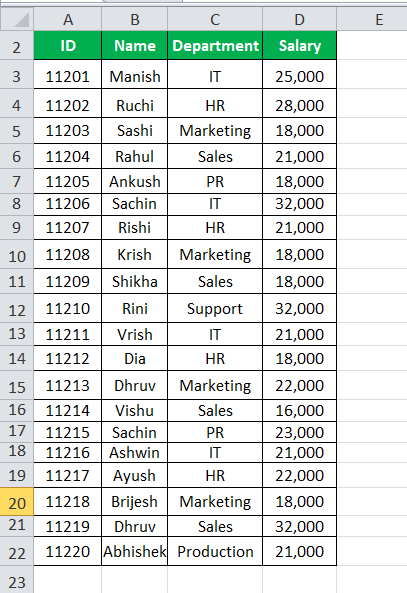
You want to look up an employee by their name and department. The search will include two details: "Name" and "Department." The name and department to look up for are given in cells G6 and G7.

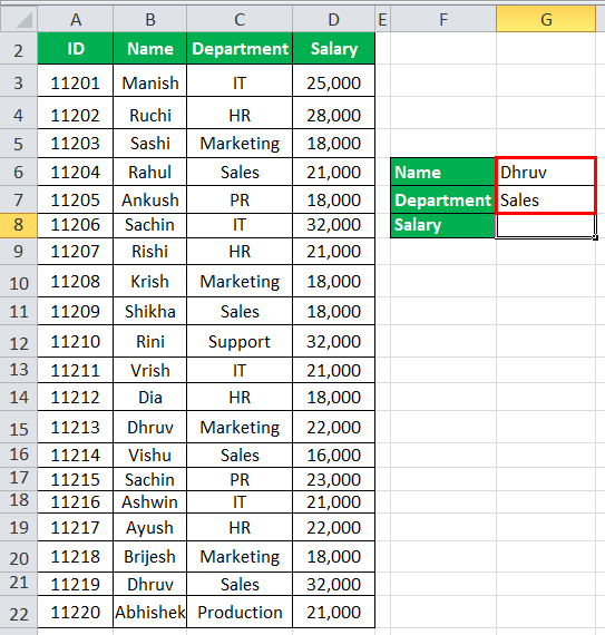
To search for "Dhruv" from the "Sales" Department, first, make a separate column containing the "Name" and "Department" of all the employees.

To do this for the first employee, use the Excel VLOOKUP Formula:

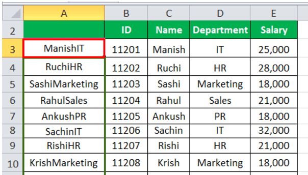
= C3 & D3

Press the "Enter" key. The cell will now contain "ManishIT." It is important to add this column to the left of the data since the first column of the array range is considered for the lookup. Now, drag it to the rest of the cells.

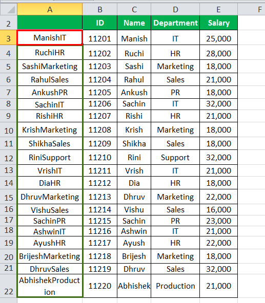
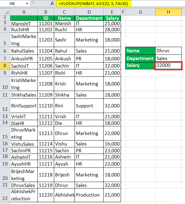
To look up the value for "Dhruv" and "Sales" given in cells G6 and G7, you can use the Excel VLOOKUP formula:

= VLOOKUP(H6 & H7, A3:E22, 5, FALSE)

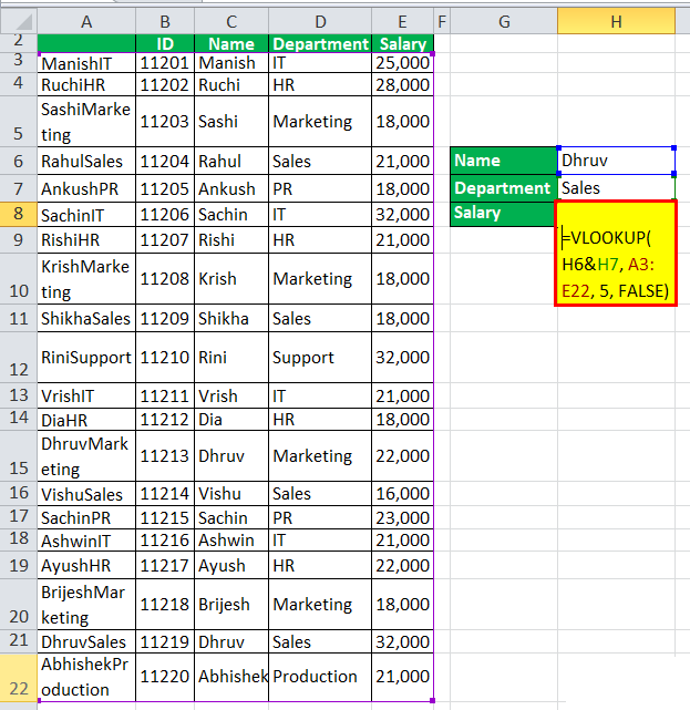
It will return the salary of the lookup employee, Dhruv, from the sales department.

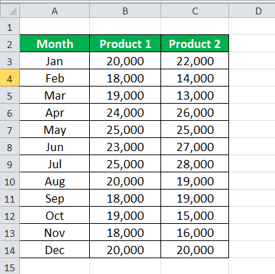
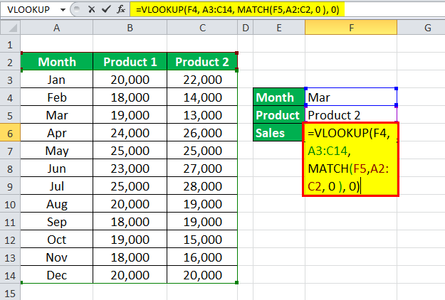
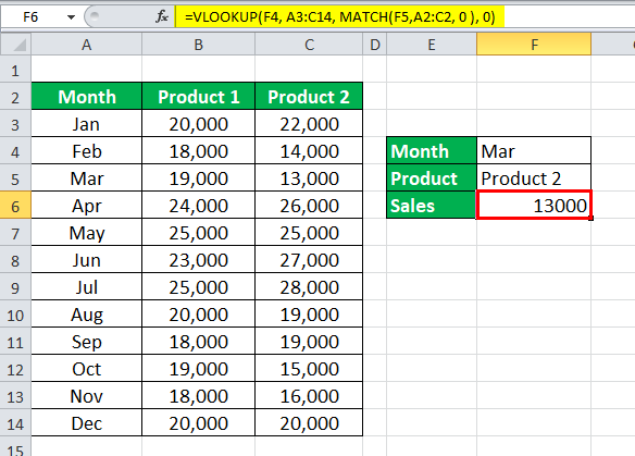
Suppose you have the sales data for two different products for 12 months, as shown below.

You want to create a lookup table in excel, in which you enter the "Month" and the "Product ID," (product 1 and product 2 in this case),which returns the sales for that product during that month.

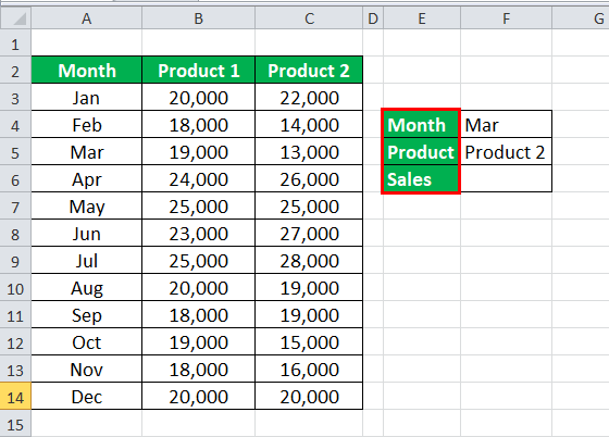
To do this, you can use the VLOOKUP and Match Formula in excel:

= VLOOKUP( F4, A3:C14, MATCH( F5, A2:C2, 0 ), 0)

The month you want to look up is given in F4, and the product name to lookup is in F5.

In this case, it will return 13,000.

Suppose you have the sales data collected for one of the products throughout the year in four different city zones, as shown below.

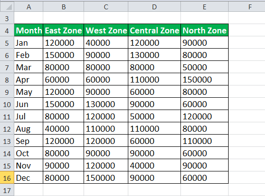
Now, you want to check if the month in which the sales were maximum for the "East Zone" is also the month in which sales were maximum for the "West Zone." To check this, first, you need to make an additional column containing the sales for the east and west zone. In this case, we separate the values by <space>.

To add the additional column to the left, use the Excel VLOOKUP formula:

= D3 & “ “ & E3

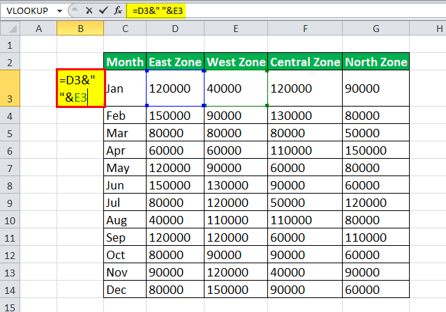
For the table's first cell, press the "Enter" key. Then, drag it to the rest of the cells.

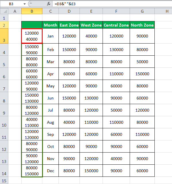
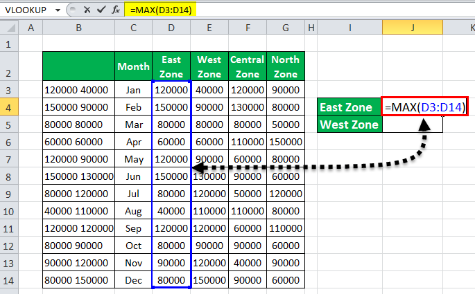
Calculate the maximum sales for "East Zone" and "West Zone" separately. To calculate the maximum value, use the Excel VLOOKUP formula:

= MAX(D3:D14) for East zone

(Learn more about the Max Function in Excel)

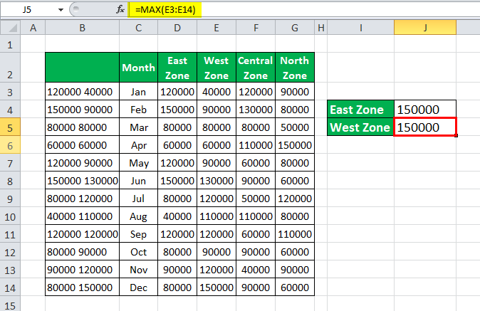
= MAX(E3:E14) for West Zone.

Now, to check if the month for which sales were maximum for the “East Zone” is also the month in which sales were maximum for the “West Zone,” you can use the following:

= IFERROR( VLOOKUP( J4 & " " & J5, B3:C14, 2, 0), "NO")

(Learn more about the IFERROR Function in Excel)

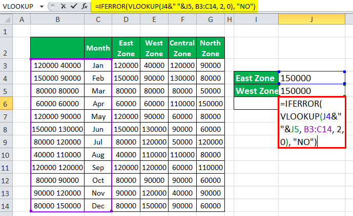
VLOOKUP( J4 &"" & J5, B3:C14, 2, 0) will search for the maximum "East Zone" and "West Zone" values in the additional column. If it can find a match, it will return the corresponding month. Else, it will give an error.

IFERROR((VLOOKUP(..)), "NO"): If the output from the VLOOKUP function is an error, it will return "NO" else. It will return the corresponding month.

Since no such month exists, let us check if the month in which the sales were maximum for the "East Zone" is the month in which the sales were second-highest for the “West Zone.” First, calculate the second-largest sales for the “West Zone” by using:

= LARGE(E3:E14, 2)

(Learn more about the LARGE Function Excel)

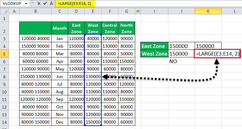
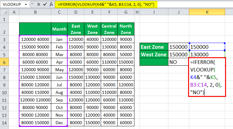
Now, use the syntax: =IFERROR(VLOOKUP(K4&" "&K5, B3:C14, 2, 0), "NO")

It will return “Jun.”

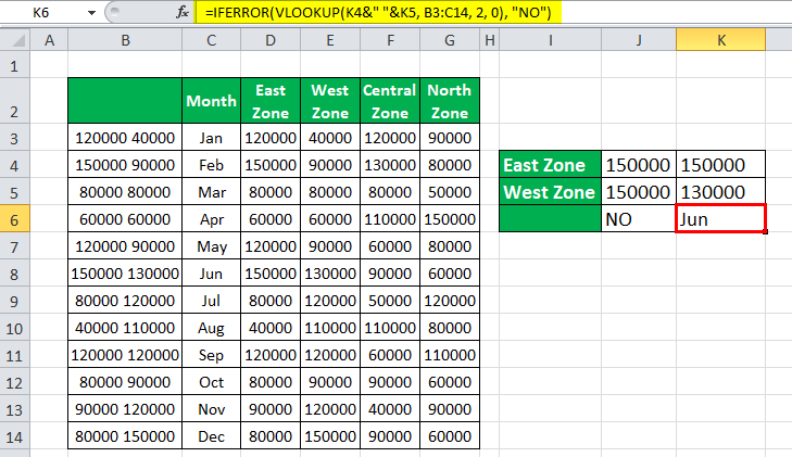
It is important to note that there can be more than one month in which the sales were maximum for the "East Zone" and "West Zone," but the Excel VLOOKUP formula will only return one of those months.

• The VLOOKUP function with multiple criteria is used to search for value in a column and return the value from a corresponding column.
• The VLOOKUP function with multiple criteria searches for the lookup_value in the first column of the given array/table.
• If you want to search the VLOOKUP function with multiple criteria, such as value1 from the first column and value2 from the second column, you need to add a column for the search. Therefore, we should add this additional column to the left of the data to appear as the first column of the lookup table.