Table Of Contents
Key Takeaways
- VLOOKUP (Vertical LOOKUP) function is used to look for values in vertical column. VLOOKUP with Two criteria is used to search for value in a column and return the value from a corresponding column.
- The VLOOKUP function with multiple criteria searches for the lookup_value in the first column of the given array/table.
- Remember, to search the VLOOKUP function with two criteria, for example, value1 from first column and value2 from second column, we need to add a column for the search.
What Is Excel VLOOKUP Two Criteria?
VLOOKUP Two Criteria in excel is used to look for value based on 2 criteria, classified commonly using ampersand.
VLOOKUP, Vertical LOOKUP is a function used to look for values in a vertical column. In fact, VLOOKUP is the most used LOOKUP function in excel.

Though VLOOKUP is useful, basic VLOOKUP function cannot help us to the full extent. need to learn advanced VLOOKUP function. This article will show you how to apply Excel VLOOKUP for two criteria.
Key takeaways
What Do Two Criteria Mean?
VLOOKUP is used to fetch the data from one table to another based on the common values available in both the tables, Lookup Value.
For example, look at the below table in the Excel worksheet.
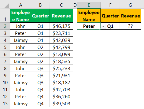
We have an employee table with the quarterly revenue they have generated. On the right-hand side, we have an employee name and quarter drop-down list in excel, so when we choose the employee name and quarter. We should get the revenue details of the selected employee for the selected quarter.
The problem with VLOOKUP here is when we apply the VLOOKUP two criteria based on employee name. We get the first value in the table for the selected employee. For example, look at the below formula applied.
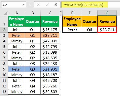
We have applied VLOOKUP for the employee “Peter” for the quarter “Q3”, but look at the result VLOOKUP has given us the “Q1” result (yellow-colored cells) instead of the “Q3” result (green-colored cells).
It is because VLOOKUP finds the first value for the “Peter” as “Q1” numbers, so it returns the same. VLOOKUP always gives the result from the first available value. So, this is where the concept of Two Criteria is important. We need to create a new column to have a unique value list.
VLOOKUP Excel Function Video Explanation
How To Create Unique Lookup Value Column?
We have duplicate names, but for each duplicate name, we have different quarter numbers. So, using these two columns, we can create a unique column called “Emp & Qtr.”
- For the column “Emp & Qtr,” we need to combine the employee name and a quarter to get a unique value column.

We have used the ampersand (&) symbol to concatenate employee names and a quarter. In addition, used underscore (_) character to differentiate employee name and quarter between employee name and quarter.
Now, we need to apply the revised VLOOKUP function to two criteria. This time lookup_value is “Emp & Qtr” instead of only the employee name.
- Open the VLOOKUP function in the H2 cell.

- Now, while choosing the lookup_value. First select the employee name cell “F2”.

- Enter concatenate symbol ampersand (&).

- In the table, we have used the underscore (_) character to separate the employee name and a quarter. So, use the same here before we select the quarter cell G2.

- Now again, put the ampersand symbol and choose quarter cell G2.

- Now, this lookup value is similar to the one we have created in the table, now choose the table array from column A to column D.
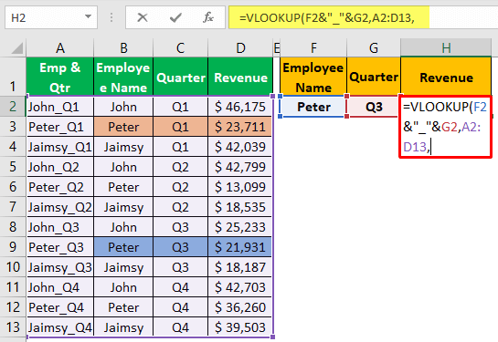
- Mention the column number from the table as 4 and range_lookup as 0 (FALSE).
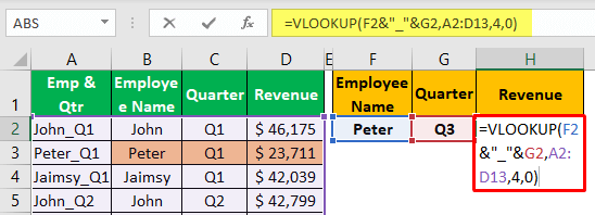
- Close the bracket and press the “Enter” key to get the result.
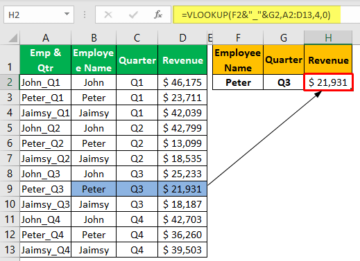
This time, we got the accurate result thanks to two criteria: helper column and lookup_value.
- We have created a dropdown list for employee names and quarters. Based on the selection from the dropdown list, it will show the revenue details for the selected employee and quarter.
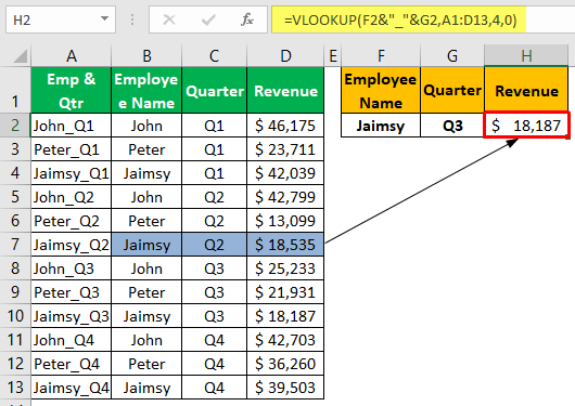
Look at the above picture. We have just changed the employee name and quarter from the dropdown list. So our formula shows the revised result accordingly.
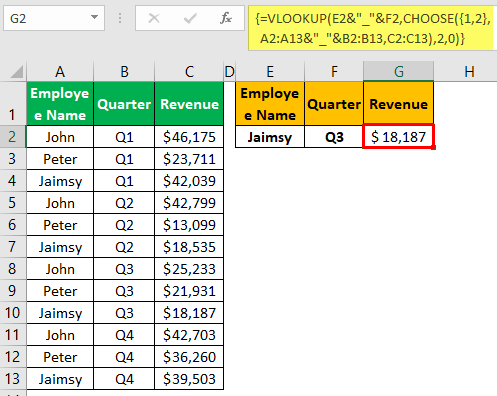
Vlookup Two Criteria Using Choose Function
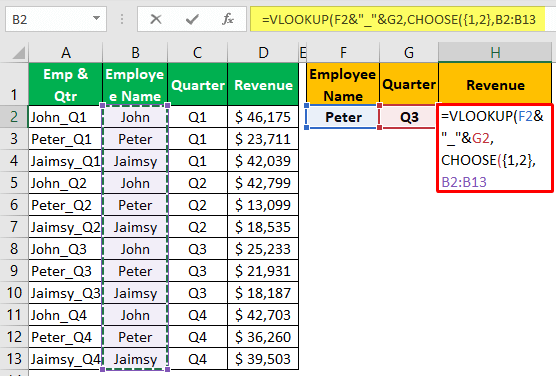
We can also use one method to match more than one criterion in VLOOKUP, using the CHOOSE function in excel.
- For this, we need not create any helper column. First, open the VLOOKUP function and select lookup values as shown above.

- For choosing Table Array, open the CHOOSE function now.
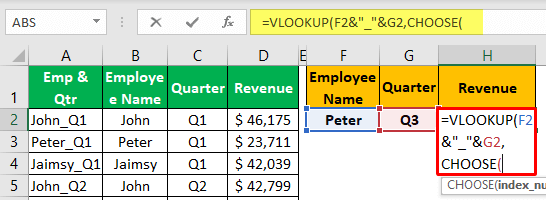
- Enter Index Number as 1, 2 in curly brackets.
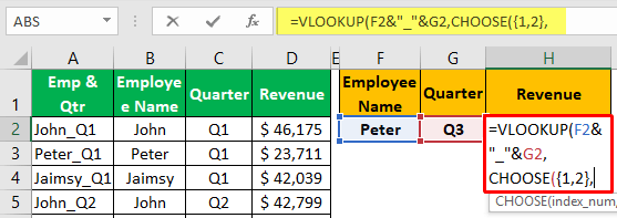
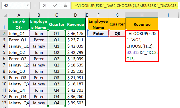
- For Value1, choose the “Employee Name” column first.
- Next, using an ampersand, combine the underscore and “Quarter” column.
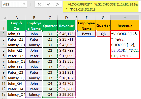
- For the Value 2 column, choose the “Revenue” column.
- We are done with the CHOOSE function to select the Table Array, close the bracket of the CHOOSE function. For column_num and range_lookup,enter as usual values.
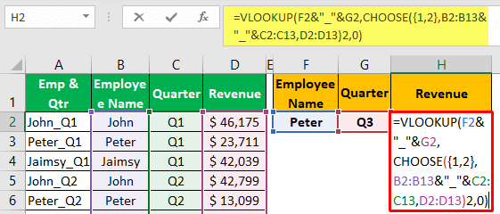
- We are done with the formula. Before we close out the formula, we must remember that this is an array too. We need to close the formula by holding three keys: “Ctrl + Shift + Enter.”
Important Things To Note
- VLOOKUP can fetch the first value found in the table for duplicate lookup values.
- Combining values will give us a unique lookup value to get an accurate result.
- Instead of using an underscore as the combining character between two values, we can use anything. The same needs to be used in the lookup_value as well.

