Vlookup to Return Multiple Values

Last Updated :

21 Aug, 2024

Blog Author :

Edited by :

Reviewed by :

Table Of Contents

Excel Vlookup to Return Multiple Values

One key functionality of the VLOOKUP function is that it will work for unique values. If there are duplicate values, then whatever is the first found value will be returned for all the other lookup values. One of the key things we need to remember while applying a VLOOKUP formula. When the lookup_value appears multiple times, we need to include different strategies if it has multiple values. This article will show you how to return multiple values using the VLOOKUP function.

Excel Vlookup to Return Multiple Values

How to Return Multiple Values using Vlookup Function?

As we have told above, VLOOKUP works for unique values. For duplicate values, it will return the first found value.

Look at the below data.

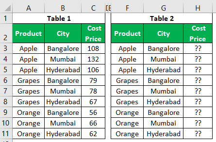
We have “Table 1” and “Table 2.” In “Table 1,” we have fruits and their prices in different cities. For “Table 2,” we need to determine the “Cost Price” from “Table 1” using the VLOOKUP function. Therefore, Apply the VLOOKUP function first.

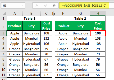
We have the same price for all the cities. For example, in “Table 1” for “Apple” in the city “Bangalore,” we have 108. Since this is the first value found in the table for “Apple,” it has returned the same for all the cities.
Similarly, for “Grapes,” the first value is 79. The same has been returned for all the cities. In the case of “Orange” also, it provides 56 for all the cities.

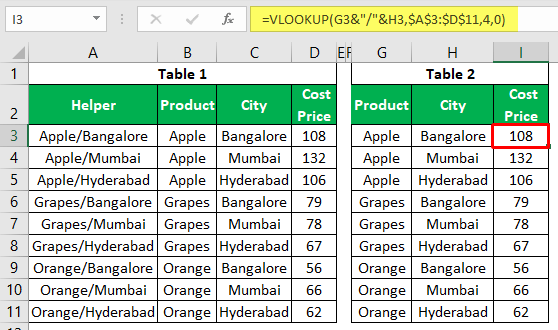
So, in these cases, we need to create a “Helper” column to create a unique lookup value list. Each fruit has different prices for each city, so a combination of fruit names and cities can create a unique list. Insert a helper column, and combine fruits and cities name.

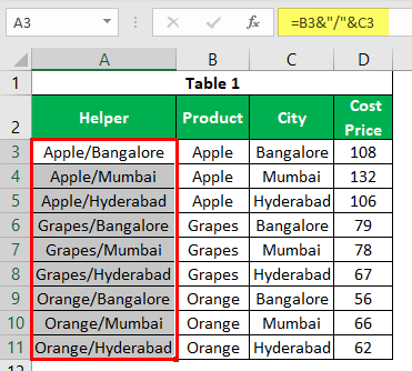
So each fruit name is combined with the city by including a backward slash (/) as the separator between fruit name and city name.

Now, return to “Table 2” and open the VLOOKUP function.

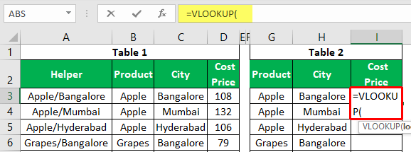
Now, we need to include the same strategy of the helper column here to choose the lookup_value. But, first, choose the fruit name.

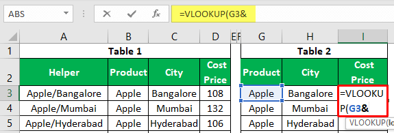
Then combine backward slash before combining with the city name.

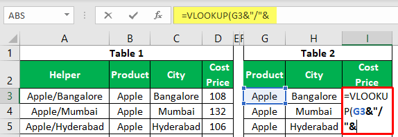
Now, combine the city name.

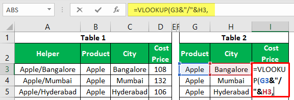
Now, the lookup_value is similar to the helper column. Now, choose the table array starting from the helper column.

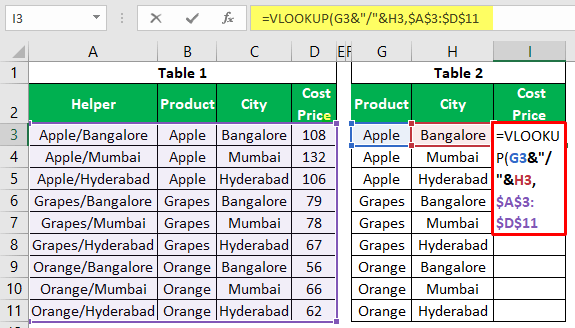
Now, mention column number 4 and range_lookup as FALSE or 0.

We have a new cost price list with accurate numbers, thanks to the helper column or the combination of fruit and city names.

VLOOKUP Excel Function - Explained in Video

Use Alternative Methods for Multiple Values

We have seen how the helper column can help fetch multiple values using the VLOOKUP formula. But imagine the situation below.

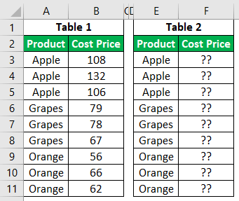
In this, we do not have any city name to create a concatenation column, so we may need to employ different strategies. Below is the complex formula we can use to get the multiple values of duplicate unique values.

=INDEX($B$2:$B$11, SMALL(IF( E3=$A$2:$A$11, ROW($A$2:$A$11)- ROW($A$2)+1), ROW(1:1)))

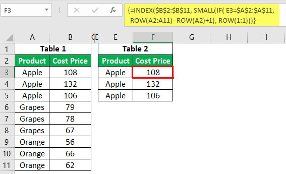
Note: The above formula is an array formula, so you must close with Ctrl + Shift + Enter.

This formula looks lengthy. However, we have another alternative method: combine the fruit name with their count on the list.

Apply the below COUNTIF function to create a helper column.

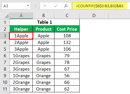
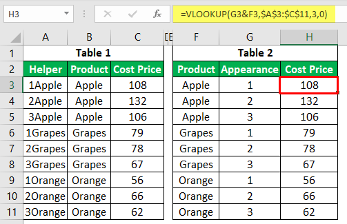
The above function will give us the count of each fruit combined with its name. For example, look at row number 4. In this, we have a count of “Apple” 2 times, so the count says 2 and combined with the fruit name gives us “2Apple”. So, this will create a unique list of fruits.

Now, create a lookup table like the below one.

Now, open the VLOOKUP function in the lookup table in the H3 cell.

The first value combined counts in the helper column, so select the numerical value and connect it with the fruit name.

Select the table and enter the column_index_number to get the result.

Things to Remember

VLOOKUP returns the same value for the lookup_values if the lookup_value has duplicate names.
To fetch multiple values of the same lookup_value, we must create helper columns using the above three methods.