VLOOKUP on Different Sheets

VLOOKUP from Different Sheets

In general, we will get data in multiple worksheets, and having all the information in single sheets is impossible in 99% of the cases. When the data is scattered to different worksheets, it isn't easy to move between sheets and pull the data from other sheets. When removing the data, VLOOKUP is vital. As a new learner, you do not have to try to fetch the data from one worksheet to another. However, this article will show you how to apply VLOOKUP to fetch the data from different sheets.

Example of VLOOKUP Function on Different Sheets

Let us recollect what the VLOOKUP formula does in general. Below is an example of how to use VLOOKUP with different sheets in Excel.

• Look at the below data in excel.

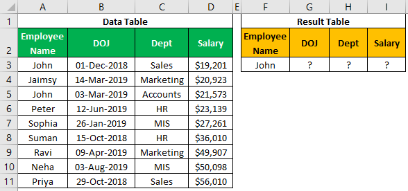
We have two tables: Data Table and Result Table.

• In the “Data Table'', we have all the values, and in the “Result Table,” we have only "Employee Name," so based on this, we need to fetch other details like “DOJ," "Dept," and "Salary.”

Below is the syntax of the VLOOKUP function.

• lookup_value: The required column in the other table is based on what value you are looking for. In this case, our lookup_value is "Employee Name."
• table _array: This is nothing but from which table we are looking for the targeted column. In this example, the table array is the data range of the Data Table in Excel.
• column _index _number: In the selected table array, we need the result from which column. To get the "DOJ," it will be the 2nd column. For "Dept," it will be the 3rd column. For the "Salary" column, it will be the 4th column.
• range_lookup: In this parameter, we must select the kind of lookup_value, i.e., either approximate or exact match. If we need an approximate match parameter, it will be "TRUE" or 1. In the case of the exact match parameter, it will be "FALSE" or 0.

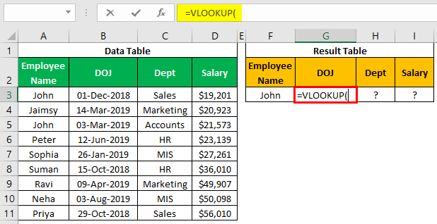
To fetch "DOJ," open the VLOOKUP function in the G3 cell.

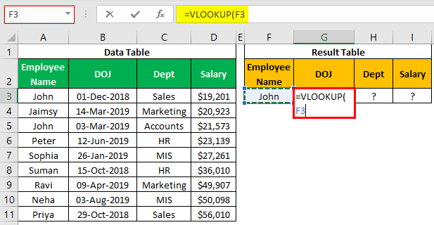
• The first argument is lookup_value, so our lookup_value is "Employee Name," so select the F3 cell.

• The table_array will be the“Data Table” range from A3 to D11.

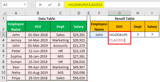
• Once you have selected the table array, make it an absolute reference by pressing the F4 key.

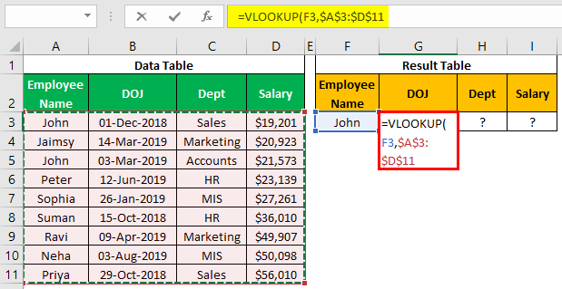
• Next is the col_index_num. So, the table array column number will be the 2nd column, so mention the same.

• Next is range_lookup. We have two options: TRUE or FALSE since we need an exact match to give the criteria as FALSE or 0.

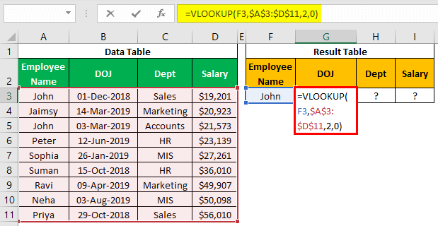
• We are done. Close the bracket and press the "Enter" key to get the result.

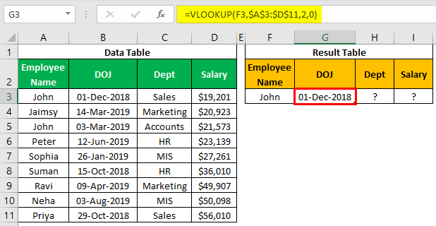
• We have "DOJ," copy the formula and paste it to the next cell. This time we need not apply the formula again. We need to change the column index number from 2 to 3.

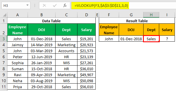
• Similarly, for the “Salary” column, change the column number to 4.

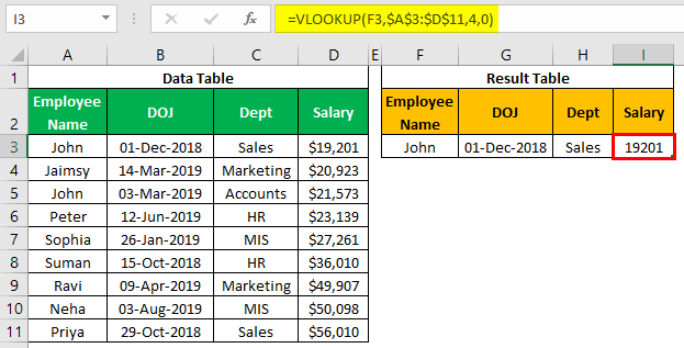
So, we have all three required details in the single formula itself. Now, we will see how to apply VLOOKUP to fetch data from one worksheet to another.

VLOOKUP Excel Video Explanation

How to Use VLOOKUP with Different Sheets on Excel?

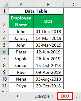
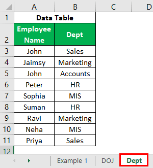
Now, we have divided the data into multiple worksheets.

#1 - DOJ Worksheet

#2 - Dept Worksheet

#3 - Salary Worksheet

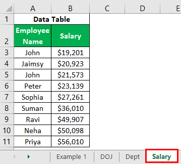
#4 - Summary Worksheet

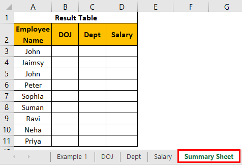
We have three pieces of information in three different worksheets, and for the “Summary Sheet,” we need to fetch the data from three other worksheets.

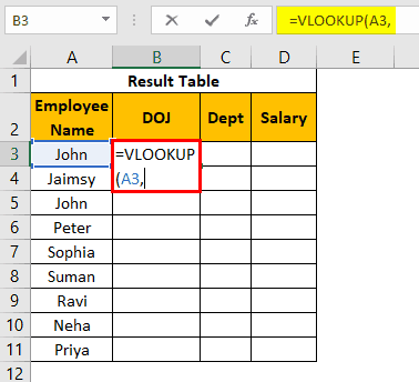
• In the "Summary Sheet," open the VLOOKUP function.

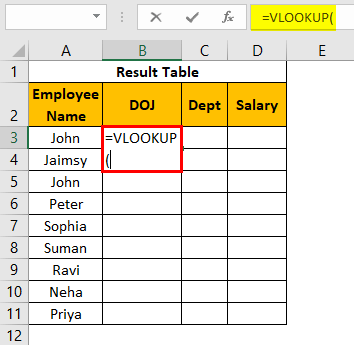
• Choose the LOOKUP value as the A3 cell.

• Since we are fetching the DOJ, for Table Array selection, go to the DOJ worksheet and choose the table range.

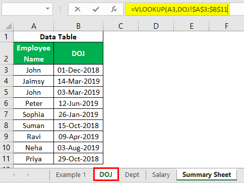
• Now, mention column number 2 and the range lookup 0.

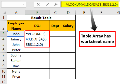
Now, the result will be: 

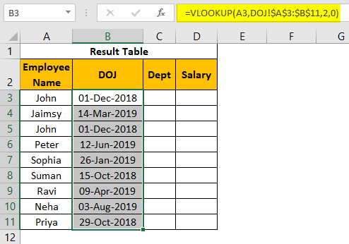
As you can see, the table array shows the worksheet name from where it is taking the reference.

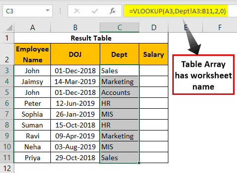
• Similarly, do the same to get "Dept" and "Salary" details. For "Dept," choose the table range from the “Dept” worksheet. For "Salary," choose the table range from the “Salary” worksheet.

• Next, do the same thing for "Salary" as well.

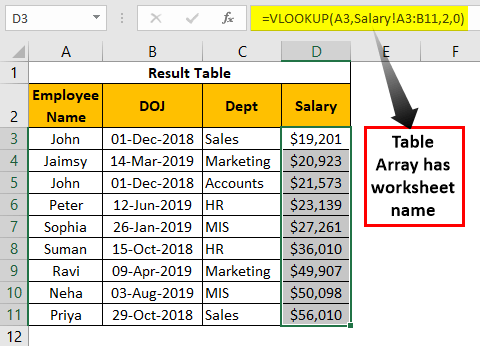
Like this, we can fetch the data from different worksheets using the VLOOKUP function.

Things to Remember Here

• While fetching the data from different worksheets using the VLOOKUP function, we must select the table array from the respective worksheet of the result-looking column.
• The lookup value should always be to the left of the required result column.
• We must always make the table array an absolute reference by pressing the F4 function key.

Recommended Articles

This article is a guide to VLOOKUP on different sheets. Here, we discuss how to fetch data from multiple Excel sheets using the VLOOKUP function, practical examples, and downloadable Excel templates. You may learn more about Excel from the following articles: -

• Vlookup to Return Multiple Values
• VLOOKUP True Criteria
• VLOOKUP Names
• Using VLOOKUP in Table Array