VBA Range

Excel VBA Range Object

Range is a property in VBA that helps specify a particular cell, a range of cells, a row, a column, or a three-dimensional range. In the context of the Excel worksheet, the VBA range object includes a single cell or multiple cells spread across various rows and columns.

For example, the range property in VBA is used to refer to specific rows or columns while writing the code. The code “Range(“A1:A5”).Value=2” returns the number 2 in the range A1:A5.

In VBA, macros are recorded and executed to automate the Excel tasks. This helps perform the repetitive processes in a faster and more accurate way. For running the macros, VBA identifies the cells on which the called tasks are to be performed. It is here that the range object in VBA comes in use.

The VBA range property is similar to the worksheet property and has several applications.

You are free to use this image on your website, templates etc, Please provide us with an attribution linkHow to Provide Attribution?Article Link to be Hyperlinked
For eg:
Source: VBA Range (wallstreetmojo.com)

How to use the VBA Range Function in Excel?

A hierarchy pattern is used in Excel VBA to refer to the range object. This three-level object hierarchy consists of the following elements:

• Object Qualifier: This refers to the location of the object. It is the workbook or the worksheet where the object is placed.
• Property: This stores the information related to the object.
• Method: This refers to the action that the object will perform. For example, for a given range, the methods are actions like sorting, formatting, selecting, clearing, etc.

The given hierarchical structure is to be followed whenever a VBA objectVBA ObjectThe “Object Required” error, also known as Error 424, is a VBA run-time error that occurs when you provide an invalid object, i.e., one that is not available in VBA's object hierarchy.read more is referred. These three elements are separated by the dot operator (.) in the following way:

Application.Workbooks.Worksheets.Range

Note 1: The range object referred by using the given (three-level) hierarchy is known as a fully qualified reference.

Note 2: The “property” and “method” are used for manipulating cell values.

The Syntax of the VBA Range Property

The syntax of the range property in VBA is shown in the following image:

For example, to refer to the cell B1 (range) in “sheet3” (worksheet) of “booknew” (workbook), the following reference is used:

Application.Workbooks(“Booknew.xlsm”).Worksheets(“Sheet3”).Range(“B1”)

Example #1–Select a Single Cell

We want to select the cell B2 in “sheet1” of the workbook.

Step 1: Open the workbook saved with the Excel extensionExcel ExtensionExcel extensions represent the file format. It helps the user to save different types of excel files in various formats. For instance, .xlsx is used for simple data, and XLSM is used to store the VBA code.read more “.xlsm” (macro-enabled workbook). The “.xlsx” format does not allow saving the macros that are presently being written.

Step 2: Open the VBA editorVBA EditorThe Visual Basic for Applications Editor is a scripting interface. These scripts are primarily responsible for the creation and execution of macros in Microsoft software.read more with the shortcut “ALT+F11.” Alternatively, click “view code” in the “controls” group of the Developer tab, as shown in the following image.

Step 3: The screen, shown in the following image, appears.

Step 4: Enter the following code.

Public  Sub SingleCellRange()
ThisWorkbook.Worksheets (“Sheet1”).Range(“B2”).Select
End Sub

With this code, we instruct the program to go to the specified cell (B2) of a particular worksheet and workbook. The action to be performed is to select the given cell.

At present, cell A2 is activated, as shown in the following image.

Step 5: Run the code by clicking “run sub/UserForm” from the Run tab. Alternatively, use the Excel shortcut key F5 to run the code.

Step 6: The result is shown in the following image. The cell B2 is selected after the execution of the program. Hence, after running the code, the activated cell is B2.

Similarly, the code can be modified to select a variety of cells and ranges and perform different actions on them.

Example #2–Select an Entire Row

We want to select the second row in “sheet1” of the workbook.

Step 1: Enter the following code and run it.

Public  Sub EntireRowRange()
ThisWorkbook.Worksheets (“Sheet1”).Range(“2:2”).Select
End Sub

The range (“2:2”) in the code represents the second row.

Step 2: The result is shown in the following image. The second row is entirely selected by running the given code.

Example #3–Select an Entire Column

We want to select the column C in “sheet1” of the workbook.

Step 1: Enter the following code and run it.

Public  Sub EntireColumnRange()
ThisWorkbook.Worksheets (“Sheet1”).Range(“C:C”).Select
End Sub

The range (“C:C”) in the code represents the column C.

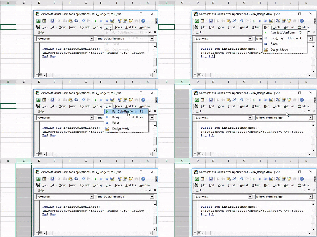
Step 2: The execution of the code and the result is shown in the following image. The column C is entirely selected by running the given code. 

Similarly, one can select contiguous and non-contiguous cells, the intersection of cell ranges, etc.

Example #4–Select Contiguous Cells

We want to select the range B2:D6 in “sheet1” of the workbook.

Step 1: Enter the following code and run it.

Public  Sub EntireColumnRange()
ThisWorkbook.Worksheets (“Sheet1”).Range(“B2:D6”).Select
End Sub

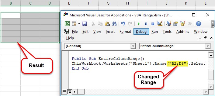
The range (“B2:D6”) in the code represents the contiguous range B2:D6.

Step 2: The result is shown in the following image. The range B2:D6 is selected by running the given code.

Example #5–Select Non-contiguous Cells

We want to select the ranges B1:C5 and G1:G3 in “sheet1” of the workbook.

Step 1: Enter the following code and run it.

Public  Sub EntireColumnRange()
ThisWorkbook.Worksheets (“Sheet1”).Range(“B1:C5, G1:G3”).Select
End Sub

The range (“B1:C5, G1:G3”) in the code represents the two non-contiguous ranges B1:C5 and G1:G3.

Step 2: The result is shown in the following image. The ranges B1:C5 and G1:G3 are selected by running the given code.

Example #6–Select a Range Intersection

We want to select the intersection of two ranges B1:G5 and G1:G3 in “sheet1” of the workbook.

Step 1: Enter the following code and run it.

Public  Sub EntireColumnRange()
ThisWorkbook.Worksheets (“Sheet1”).Range(“B1:G5 G1:G3”).Select
End Sub

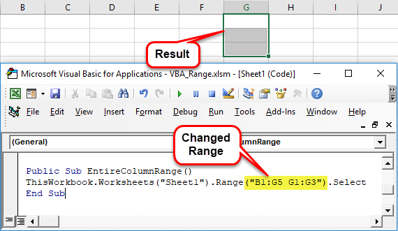
The range (“B1:G5 G1:G3”) in the code represents the intersection of the two ranges B1:G5 and G1:G3.

Note: The comma within the two ranges is absent in this case.

Step 2: The result is shown in the following image. The cells common to the ranges B1:G5 and G1:G3 are selected by running the given code. Hence, the common cells in the specified range are G1:G3.

Example #7–Merge a Range of Cells

We want to select and merge the cells B1:C5 in “sheet1” of the workbook.

Step 1: Enter the following code and run it.

Public  Sub MergeRange()
ThisWorkbook.Worksheets (“Sheet1”).Range(“B1:C5”).Merge
End Sub

The range (“B1:C5”) represents the range B1:C5 on which we are performing the action “merge.”

Step 2: The result is shown in the following image. The cells in the range B1:C5 have been merged by running the given code.

Example #8–Clear Formatting of a Range

The following image shows the range F2:H6, which is highlighted in yellow. We want to clear the Excel formattingExcel FormattingFormatting is a useful feature in Excel that allows you to change the appearance of the data in a worksheet. Formatting can be done in a variety of ways. For example, we can use the styles and format tab on the home tab to change the font of a cell or a table.read more on this range in “sheet1” of the workbook.

Step 1: Enter the following code and run it.

Public  Sub ClearFormats()
ThisWorkbook.Worksheets(“Sheet1”).Range(“F2:H6”).ClearFormats
End Sub

The range (“F2:H6”) in the given syntaxSyntax:VBA ThisWorkbook refers to the workbook on which the users currently write the code to execute all of the tasks in the current workbook. In this, it doesn't matter which workbook is active and only requires the reference to the workbook, where the users write the code.read more represents the range F2:H6 from which we are removing the existing formatting.

Step 2: The result is shown in the following image. The formatting from the cells in the range F2:H6 has been cleared by running the given code.

Similarly, the formatting of the entire worksheet can be removed. Moreover, the content of a range of cells can be cleared by using the action “.ClearContents.”

Frequently Asked Questions

Recommended Articles

This has been a guide to VBA Range. Here we learn how to select a particular cell and range of cells with the help of VBA range objects and examples in Excel. You may also have a look at other articles related to Excel VBA –

• VBA Application.Match
• Excel VBA Cells Reference
• Use VLookup in VBA
• Using VBA Msg Box