VBA Filter Data

VBA Filter tool one can use to sort out or fetch the specific data desired. For example, one can use the Autofilter function as a worksheet function. However, this function has other arguments with it which are optional, and the only mandatory argument is the expression that covers the range. For example, worksheets("Sheet1").Range("A1").Autofilter will apply the filter on the first column.

Filter in VBA works the same way it works in the worksheet. The only thing different is we can automate the routine task of filtering the data through coding.

The AutoFilter is a function that includes many syntax values. Below are the parameters involved in the AutoFilter function.

• The range is the first thing we need to supply to use the "AutoFilter" option. After that, it is simply for which range of cells we need to apply the filter, for example, Range ("A1:D50").
• The field is the first argument in the function. Once we select the range of cells through the VBA RANGE object, we need to mention for which column of the range we want to apply the filter for.
• Criteria 1 is nothing, but in the selected Field, the value that you want to filter out.
• The operator we may use if we want to use the Criteria 2 argument. In this option, we can use the below options.
  xlAnd, xlOr, xlBottom10Items, xlTop10Items, xlTop10Percent, xlBottom10Percent, xlFilterCellColor, xlFilterDynamic, xlFilterFontColor, xlFilterIcon, xlFilterValues
• Visible Dropdown displays a filter symbol in the filter applied column. If you want to display it, you can supply the argument as TRUE or else FALSE.

Example #1 - Apply or Remove Filter to the Data

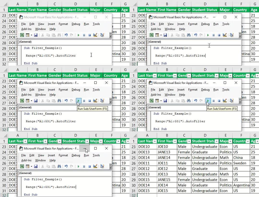
If you want to apply the filter option to the data, then we can turn it off and on this option. For example, look at the below data image.

Step 1: Supply data range

To activate the filter option first, we need to supply what is our data range. For example, in the above image, our data is spread from A1 to G31. So, supply this range using a RANGE object.

Code:

Sub Filter_Example()

  Range ("A1:G31")

End Sub

Step 2: Then access AutoFilter function

Now, access the AutoFilter function for this range.

Code:

Sub Filter_Example()

  Range("A1:G31").AutoFilter

End Sub

Step 3: Run the code to enable the filter

That is all. Run this code to enable the AutoFilter.

This code works as a toggle. If the filter is not applied, it will apply. If already applied, then it will be removed.

Example #2 - Filter Specific Values

Now, we will see how to use the parameters of the AutoFilter option. Take the same data as above. For example, we must filter out all "Male" gender names.

Step 1: Select Range and Open Autofilter Function

Step 2: Then Select Field

In the function's first argument, i.e., Field, we need to mention the column reference we would like to filter out. In this example, we need to filter only “Male” candidates, column “C,” so the column number is 3.

Step 3: Now Mention Criteria

Now for this supplied Field, we need to mention  Criteria 1, i.e., what value we need to filter in the  Field. We need to filter “Male” from this column.

Code:

Sub Filter_Example()

  Range("A1:G31").AutoFilter Field:=3, Criteria1:="Male"

End Sub

Step 4: And run the code

Ok, that’s all. So this code will filter only “Male” candidates now.

Example #3 - Usage of OPERATOR Argument

When you want to filter out more than one value from the column, we need to use the “Operator” argument. For example, from the column “Major,” we need to filter only “Math & Politics,” then we need to use this argument.

Step 1: Select Range and Autofilter Field

First, supply the Range of cells and fields.

Code:

Sub Filter_Example()

 Range("A1:G31").AutoFilter Field:=5,

End Sub

Step 2: Enter Criteria 1 as Math

For the mentioned field, we need to supply Criteria 1 as "Math."

Code:

Sub Filter_Example()

 Range("A1:G31").AutoFilter Field:=5, Criteria1:="Math",

End Sub

Step 3: Use Operator xl

Since we need to filter one more value from the same column or field, use the operator symbol as "xlOr."

Code:

Sub Filter_Example()

  Range("A1:G31").AutoFilter Field:=5, Criteria1:="Math", 
  Operator:=xlOr

End Sub

Step 4: Enter Criteria 2 as Politics

And for Criteria 2 argument, mention the value as "Politics."

Code:

Sub Filter_Example()

 Range("A1:G31").AutoFilter Field:=5, Criteria1:="Math",
 Operator:=xlOr, Criteria2:="Politics"

End Sub

It will filter out both "Math" and "Politics" from column "Major."

Example #4 - Filter Numbers with Operator Symbols

For example, if you want to filter numbers, we can filter a specific number and numbers above, below, or between specific values and a range of values.

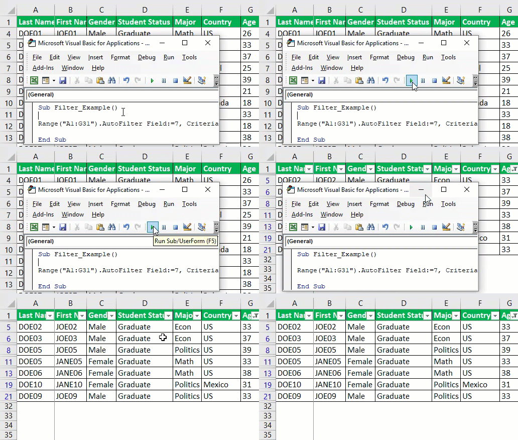
For example, if you want to filter persons aged more than 30, then we can write the code below from the age column.

Code:

Sub Filter_Example()

 Range("A1:G31").AutoFilter Field:=7, Criteria1:=">30"

End Sub

It will filter all the values that are more than 30.

Now, if you want to filter values between 21 and 31, we can use the code below.

Code:

Sub Filter_Example()

 Range("A1:G31").AutoFilter Field:=7, Criteria1:=">21", 
 Operator:=xlAnd, Criteria2:="<31"

End Sub

It will filter persons aged between 21 and 30.

Example #5 - Apply Filter for More Than One Column

We need to use a slightly different technique if you want to filter values from more than one column criteria.

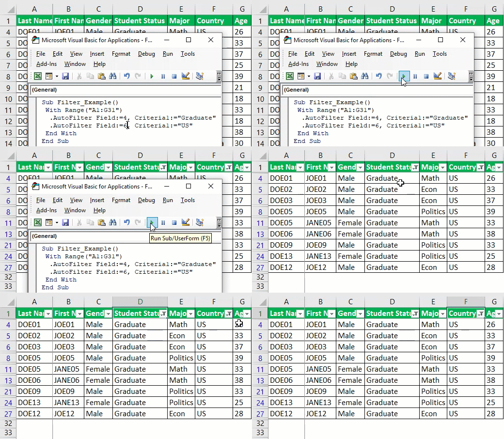
If you want to filter "Student Status" as "Graduate" and "Country" as "US," then first, we need to supply the RANGE of cells under the WITH statement.

Code:

Sub Filter_Example()

  With Range("A1:G31")

  End With

End Sub

Inside the WITH statement, supply the first criteria to be filtered.

Code:

Sub Filter_Example()

 With Range("A1:G31")
  .AutoFilter Field:=4, Criteria1:="Graduate"
 End With

End Sub

Now, in the next line, do the same for "Country" by changing "Field" to six and "Criteria" to "US."

Code:

Sub Filter_Example()

 With Range("A1:G31")
  .AutoFilter Field:=4, Criteria1:="Graduate"
  .AutoFilter Field:=6, Criteria1:="US"
 End With

End Sub

Now, this will filter "Graduate" only for the country "US."

• It will apply the first thing only for the mentioned range of cells filter.
• The field is nothing in which column you want to filter the data.
• If filtering values from more than one column, use the With statement.