TYPE Excel Function

What Is TYPE Excel Function?

The TYPE Excel function is an inbuilt Information function that accepts one value at a time and returns the data type of the specified value as a numeric code.

Users can utilize the TYPE Excel function in formulas, which work based on the input value type in a cell. Also, the function is useful for determining the data types a function or formula accepts and returns.

For example, the following dataset contains a list of values.

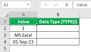
The requirement is to update the listed values’ types as numeric codes in column B.

Then, we can determine each value’s data type Excel numeric code in the corresponding target cell using the TYPE function.

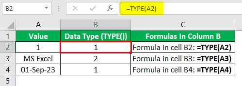
In the above data type Excel example, the TYPE() in each target cell accepts the cell reference to the value in the corresponding row. It then returns the data type of the supplied value as a numeric code.

Excel considers integers and dates as a Number type with the numeric code of 1 and a word as a Text type with a numeric code of 2. Thus, the TYPE Excel formula returns the data type as the numeric code 1 in cells B2 and B4 and the numeric code 2 in cell B3, respectively.

• The TYPE Excel function accepts one value and returns its data type numeric code.
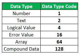
• The numeric codes of the data types Number, Text, Logical Value, Error Value, Array, and Compound Data the TYPE() returns are 1, 2, 4, 16, 64, and 128, respectively.
• Users can utilize the TYPE function to determine the data type of the value a formula accepts as an input and returns as the output.
• Using the TYPE function with other inbuilt functions such as IF, CHOOSE, and MIN yields productive results.

Syntax

The TYPE Excel formula syntax is as follows:

Where,

• value: The data for which we want the TYPE Excel function to determine the type. The argument value can be a value or a cell reference to the value. However, if the argument value is a formula or a cell reference to the formula, the TYPE() output is the type of the value the formula returns.

Use the table below to check data type Excel codes the TYPE function can return based on the input value.

How To Use TYPE Excel Function?

While we can use data type Excel VBA to obtain the required data type numeric code of the given value, we shall see the more straightforward methods.

We can utilize the TYPE Excel function in two ways:

1. Access from the Excel ribbon.
2. Enter in the worksheet manually.

Method #1 – Access From The Excel Ribbon

Select a target cell for output - The Formulas tab - The More Functions option down arrow - The Information option right arrow - The TYPE Excel function, as shown below.

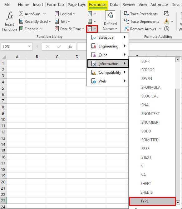
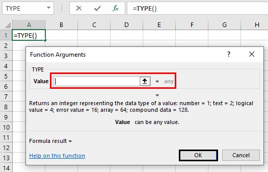
The Function Arguments window will open. Enter the argument in the Value field and click OK to check data type Excel of the specified value in the target cell, as depicted below.

Method #2 – Enter In The Worksheet Manually

1. Choose a target cell for the output.
2. Type =TYPE( in the cell.
3. Enter the argument as a cell value or reference and close the brackets.
4. Press Enter to execute the TYPE Excel function and obtain the required data type numeric code.

Examples

Check out the TYPE Excel function examples to use it effectively.

Example #1

The below dataset contains a list of values and descriptions to determine the data type codes based on the listed values.

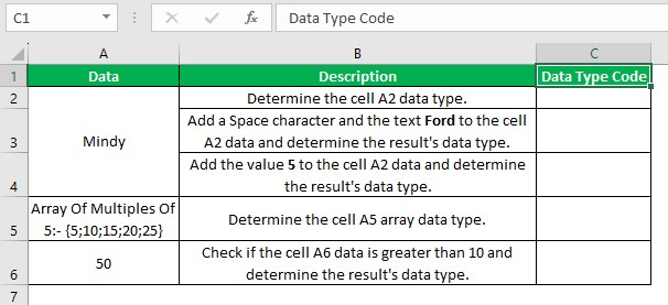
Assume we must display the required data type codes in column C

Then, while we can use the data type Excel VBA macros to determine the required values in the target cells, let us see the more straightforward methods.

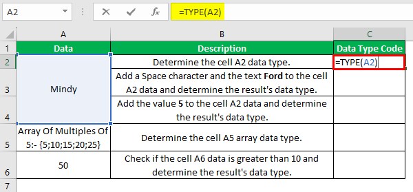
Step 1: Select cell C2 and enter the TYPE Excel function.

=TYPE(A2)

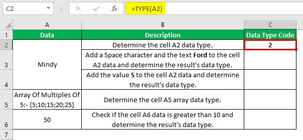
Step 2: Press Enter to view the TYPE Excel function.

Step 3: Choose cell C3, enter the TYPE(), and press Enter.

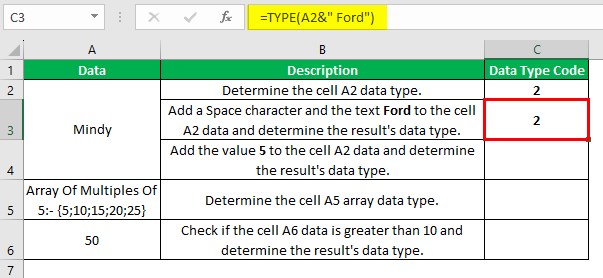
=TYPE(A2&" Ford")

Step 4: Choose cell C4, enter the TYPE(), and press Enter.

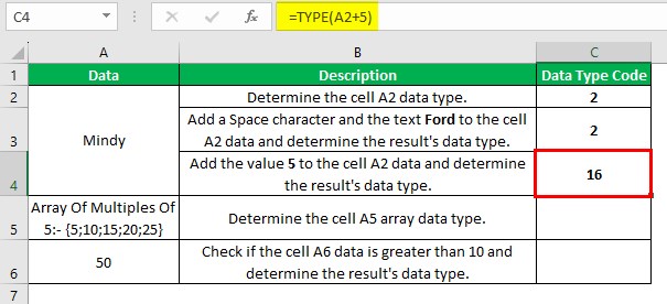
=TYPE(A2+5)

Step 5: Choose cell C5, enter the TYPE(), and press Enter.

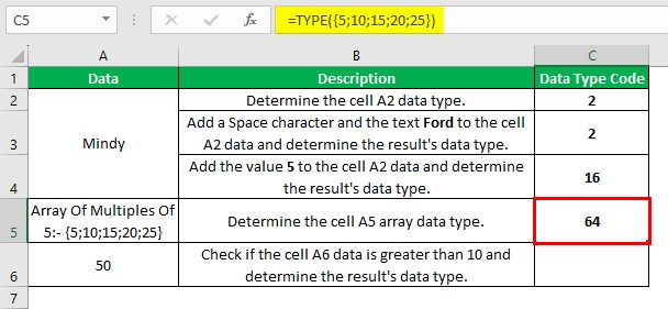
=TYPE({5;10;15;20;25})

Step 6: Choose cell C6, enter the TYPE(), and press Enter.

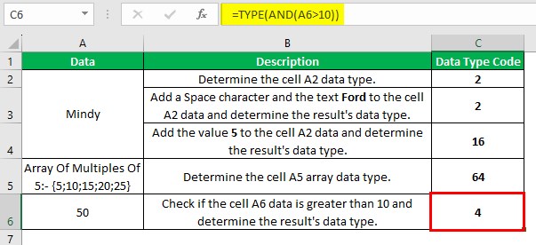
=TYPE(AND(A6>10))

In the above example, the input values in the cells C2:C3 formulas are texts, leading to the TYPE() in the two cells returning the Text data type code, 2.

Next, adding a number 5 to the cell A2 text returns the Excel #VALUE! error value. Thus, the TYPE() in cell C4 returns the error value data type code 16.

On the other hand, the cell C5 TYPE() accepts an array value and returns its data type code, 64.

Finally, the cell C6 formula checks if the cell A6 value is greater than 10 in the AND Excel function. Since the condition holds, the AND() returns the logical value TRUE. Thus, the TYPE() returns the logical value data type code, 4.

Example #2

The following data set contains an employee’s data.

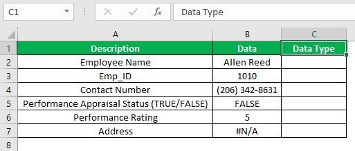
The aim is to determine the data type of the values in the employee data range and display the output in column C. Then, we can apply the TYPE Excel function with the IF Excel function in the target cells to achieve the desired output.

Step 1: Choose cell C2, enter the IF() containing the TYPE(), and press Enter.

=IF(TYPE(B2)=1,"Number",IF(TYPE(B2)=2,"Text",IF(TYPE(B2)=4,"Logical Value",IF(TYPE(B2)=16,"Error Value",""))))

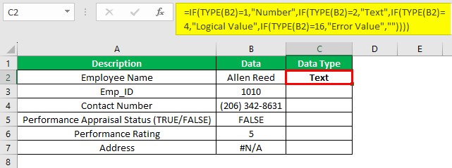
Step 2: Using the Excel fill handle, update the TYPE Excel function in the remaining target cells.

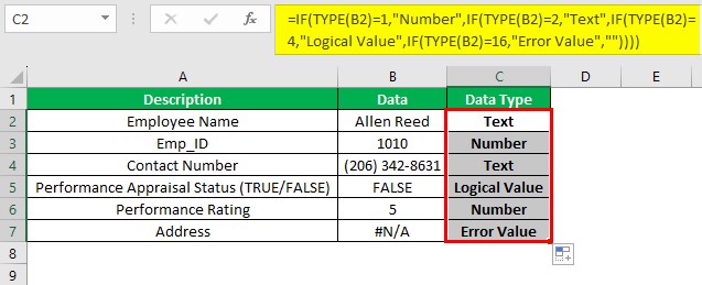
Let us check the cell C7 formula to understand the logic.

The first TYPE() returns the cell B7 value’s type, 16, since cell B7 contains an error value. Thus, the outer-most IF() condition does not hold, and the function returns the FALSE value.

The FALSE value is again an IF(). It checks if the TYPE(B7) output is 2. Since the IF condition does not hold, the IF() output is the FALSE value. Next, the IF() in the FALSE value checks of the TYPE(B7) output is 4. Again, the IF() condition is false, leading to the function returning the FALSE value.

The last IF() checks if the TYPE(B7) output is 16. This time the condition holds, leading to the IF() returning the TRUE value, “Error Value”, as the cell B7 data type.

Example #3

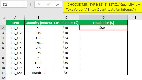
The following dataset lists items, their quantities and cost per box data.

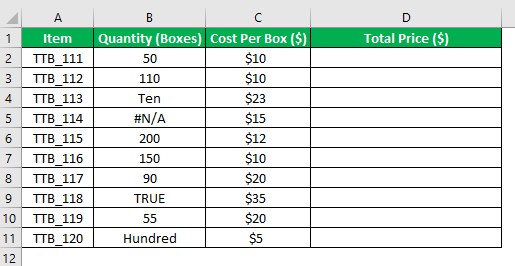
The requirement is to update the total cost values for all the items in column D, with columns C and D having the same data type.

However, a few column B cells show values that are not integers. Thus, we can use the CHOOSE, MIN, and TYPE Excel functions-based formula in each target cell to achieve the required output.

Step 1: Choose cell D2, enter the following formula, and press Enter.

=CHOOSE(MIN(TYPE(B2),3),B2*C2,"Quantity Is A Text Value.","Enter Quantity As An Integer.")

Step 2: Use the fill handle to implement the formula in the remaining target cells.

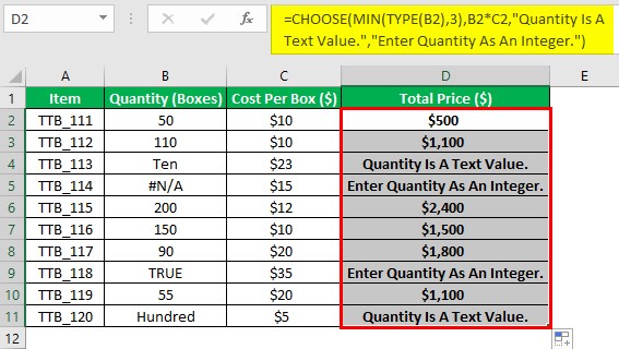
Let us check the cell D11 formula to understand the logic.

First, the TYPE() returns the cell B11 data type code, 2. Next, the Excel MIN function returns the least value out of 2 and 3, which is 2. Thus, the Excel CHOOSE function returns the text value “Quantity Is A Text Value.”, based on the index number 2.

Important Things To Note

• Supply only one value or cell reference to one value as the argument value to the TYPE Excel function. Otherwise, the function will fail to execute.
• If we refer to a blank cell as the TYPE() argument value, the function output will be 1.
• When the supplied argument value to the TYPE() is a formula or cell reference to the formula, the TYPE() returns the data type of the formula output.

Frequently Asked Questions (FAQs)

Download Template

This article must be helpful to understand the TYPE Excel, with its formula and examples. You can download the template here to use it instantly.

Recommended Articles

This has been a guide to What Is TYPE Excel. Here we learn the TYPE Excel function syntax and how to use it with examples and points to remember. You can learn more from the following articles –

• IFERROR Excel Function
• Concatenate Excel Function
• Match Excel Function