Table Of Contents
Trim Function In Excel
TRIM in Excel is a text function that removes unwanted space, like extra space in-between the words or at the beginning and end of the sentences or words. This formula does not remove if a single space is present between two words.
TRIM function in Excel is an inbuilt text function, so we can insert the formula from the “Function Library” or enter it directly in the worksheet.
For example, suppose we have a name in cell A1 containing some whitespace before and after the text, and more than one space between the words, as “ John Wright ”.

The output is “John Wright” after applying the TRIM formula as =TRIM(A1), as shown above in cell B1.
Key Takeaways
- The TRIM in Excel removes extra spaces from the text, leaving no extra space between words and at the beginning and end of the string.
- It can only remove the ASCII space character (32) from text/string.
- It cannot remove the Unicode text that often contains a non-breaking space character (160) that appears on web pages as the HTML entity.
- This function is useful for refining the text from other applications or environments.
- We can use TRIM with other Excel functions such as LEN(), SUBSTITUTE(), etc.
Syntax Of Excel TRIM Formula
The syntax of the TRIM formula is,

The TRIM formula in Excel has only one critical parameter: text.
- text: it is a text from which you want to remove extra spaces.
How To Use TRIM Function In Excel?
We can use the TRIM Excel function in 2 ways, namely:
- Access from the Excel ribbon.
- Enter in the worksheet manually.
Method #1 – Access from the Excel ribbon
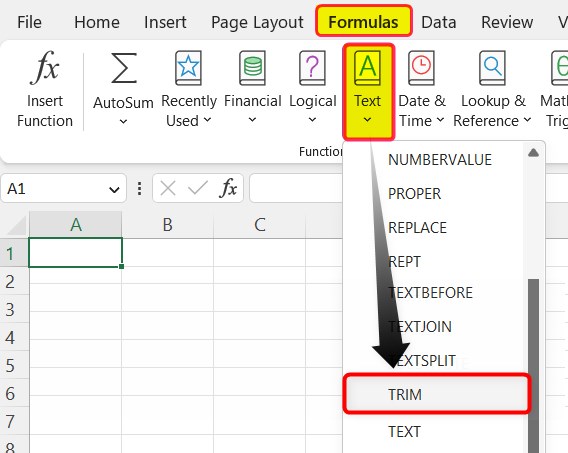
Choose an empty cell for the result à select the “Formulas” tab à go to the “Function Library” group à click the “Text” option drop-down à select the “TRIM” function, as shown below.
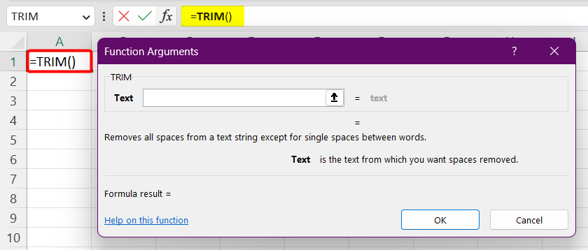
The “Function Arguments” window appears. Enter the arguments in the “Text” field, and click “OK”, as shown below.
Method #2 – Enter in the worksheet manually
- Select an empty cell for the output.
- Type =TRIM( in the selected cell. [Alternatively, type =T or =TR and double-click the TRIM function from the list of suggestions shown by Excel.
- Enter the argument as cell value or cell reference and close the brackets.
- Press the “Enter” key.
Basic Example
Let us understand the working of the TRIM function in Excel using an example.
.
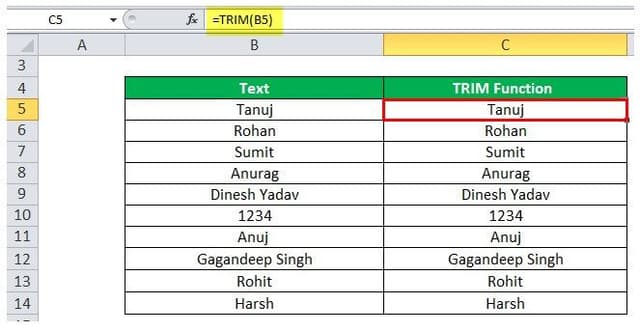
In this example, the TRIM function in Excel removes the extra spaces from the given texts/ words at the beginning and end.
Select cell C5, enter the formula =TRIM(B5), press “Enter”, and drag the formula from cell C5 to C14 using the fill handle.
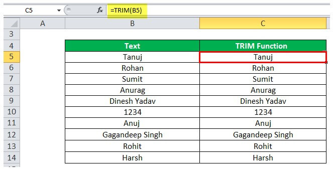
The output is shown above. So, for example, applying TRIM on “ Tanuj ”, the output will be “Tanuj” without the spaces.
Examples
We will consider some scenarios using the TRIM Excel function examples.
Example #1
In this example, the trim removes the extra spaces from the middle of the given text string, as shown in the below table.
Select cell C19, enter the formula =TRIM(B19), press “Enter”, and drag the formula from cell C19 to C26 using the fill handle.

The output is shown above. For example, in cell C19, “Note that the Trim function is similar to” becomes “Note that the Trim function is similar”.
Example #2
In the following example, to calculate the number of words in cell B1 string – “Note that the Trim function is similar”.
- Here, we can use the formula =LEN(B31)-LEN(SUBSTITUTE(B31,”,”))+1. However, it will count the number of spaces and add one to it. But if there are extra spaces between the string, it will not work, so we use trim to achieve it.
- Therefore, select cell C32, enter the formula =LEN(TRIM(B32))-LEN(SUBSTITUTE(B32,” “,”))+1 function, press “Enter”, and drag the formula from cell C32 to C39 using the fill handle.
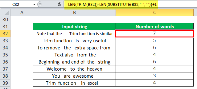
The output is shown above. The formula will remove extra spaces, then count the number of spaces and add one to give the total number of words in the string.
Example #3
We can use Excel’s TRIM and substitute function in excel to join the multiple columns separated by a comma.
Select cell J5, enter the TRIM formula =SUBSTITUTE(TRIM(F5&” “&G5&” “&H5&” “&I5),” “,”, “), press “Enter”, and drag the formula from cell J5 to J12 using the fill handle.
The output is shown above.
Important Things To Note
- We can use the TRIM formula only for text strings in words, names, sentences, etc.
- If the cell value or cell reference is numeric or alpha-numeric, then the output will be the exact same value as the selected value.
