TEXTJOIN Excel

What Is TEXTJOIN Function In Excel?

The TEXTJOIN Excel function is an inbuilt Text function. It combines multiple text strings from different cells or ranges, with the values separated by the specified delimiter.

Users can utilize the TEXTJOIN Excel function to merge complex financial and statistical data in a cell. Also, the function helps users prepare massive client and customer email lists required for productive marketing strategies.

For example, the following dataset shows four text strings in each row, with column A providing the corresponding descriptions.

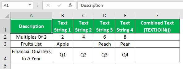
The requirement is to merge the four text strings in each row to show a combined text separated by a comma and space in column F cells.

Then, considering the TEXTJOIN Excel definition, we can apply the TEXTJOIN() in the target cells to achieve the required outcome.

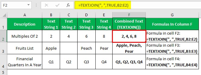
In the above TEXTJOIN Excel example, we supply three argument values to the TEXTJOIN().

The first argument is the delimiter we want to display between the text strings in the combined text. It is a comma followed by a space character in this case. Next, we set the second argument as TRUE to ignore empty cells in the range containing the text strings to merge we supply as the third argument.

Thus, the TEXTJOIN Excel in each target cell merges the four text strings specified in the corresponding row with the cited delimiter between the values.

Furthermore, in the case of the cell F3 TEXTJOIN Excel function, the function ignores the empty cell C3 and combines the remaining three text strings to return the required output.

• The TEXTJOIN Excel function is an inbuilt function that concatenates the given text strings, separated by the specified delimiter. The source text strings and one or more delimiters can be in cells or ranges.
• Users can utilize the TEXTJOIN function to display massive sets of data, separated by delimiters, as a list in one cell.
• We can apply the TEXTJOIN function by directly entering it into a cell or from the Formulas tab. The function accepts three mandatory arguments, delimiter, ignore_empty, and text1, and 251 optional text arguments.
• While we can apply the TEXTJOIN() as a standalone function, using it with other inbuilt functions, such as IF and TEXT, helps achieve practical results.

Syntax

Firstly, the TEXTJOIN Excel 2016 is unavailable, and we can use the function only from Excel 2019 onwards. So, when we try applying the function in the Excel versions before 2019, we face the #NAME? error.

The TEXTJOIN Excel function syntax is as follows:

Where,

• delimiter: A text string that must appear between the text strings we aim to join. It can be empty, a text string or an array of multiple characters within double quotations, a reference to a cell having a valid text string or a range containing text strings. And if the TEXTJOIN Excel delimiter argument is a number, the function recognizes it as a text value.
• ignore_empty: The argument value is logical. It is TRUE if the function must ignore empty cells and FALSE if it must include empty cells when combining text strings.
• text1: It is a text string or an array of text strings in double quotes, a reference to a cell holding a text string or a range containing strings we aim to combine.
• text2,…: The remaining text values we want to join. However, the function can accept up to 252 text argument values, including text1. Also, the output character limit is 32,767, which, when exceeded, leads to the function returning the #VALUE! error.

While the first three arguments in the TEXTJOIN Excel function are mandatory, the remaining are optional. Also, if we do not supply the TEXTJOIN Excel delimiter argument value or it is an empty string, the text strings merge without a delimiter.

How To Use TEXTJOIN Function In Excel?

We can use the TEXTJOIN Excel function using the following two methods:

1. Access from the Excel ribbon.
2. Enter into the worksheet manually.

Method #1 – Access From The Excel Ribbon

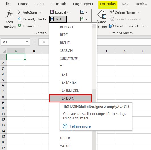
Select a target cell for output - choose the Formulas tab - click the Text group functions down arrow - select the TEXTJOIN Excel function, as depicted below.

The Function Arguments window will open. Enter the mandatory function arguments in the Delimiter, Ignore_empty, and Text1 fields.

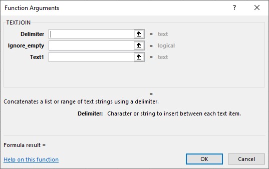
Further, clicking in the Text1 field will show the option field, Text2, where we can enter another text string. Likewise, clicking in each Text field will show the next text field, which we can use to enter the subsequent text strings to join.

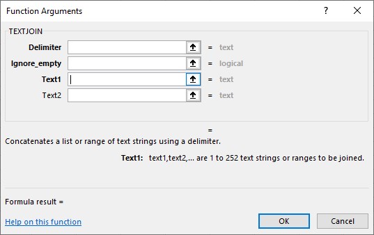
Click OK in the Function Arguments window to exit it and view the required joined text value in the target cell.

Method #2 – Enter Into The Worksheet Manually

1. Select a target cell for the output.
2. Type =TEXTJOIN( in the cell.
   However, we cannot find TEXTJOIN Excel 2016. It is available in the Excel 2019 and the latest versions.
3. Enter the cell values and references as the argument values. Ensure to supply the text strings in double quotes if supplying them directly as the respective argument values.
4. Close the brackets and press Enter to view the combined text value as the TEXTJOIN Excel function output in the target cell.

Examples

Check out the following examples to understand the TEXTJOIN Excel definition and use the function effectively.

Example #1

We shall see how to merge text strings with different delimiters using the TEXTJOIN Excel function.

The following image shows two datasets. While the first one contains students’ first, middle, and last names, the second shows a set of delimiters.

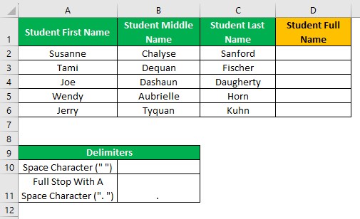
The aim is to display the students’ full names by joining each student’s first, middle, and last names, with a space between the first name and the first letter of the middle name. Next, we must display a full stop and a space character as the delimiter between the first letter of the middle name and the last name. Assume column D cells are the target cells.

Then, here is how to use the TEXTJOIN Excel function in the target cells to achieve the required output.

Step 1: Choose cell D2 and enter the following TEXTJOIN().

=TEXTJOIN({" ",". "},TRUE,A2,LEFT(B2,1),C2)

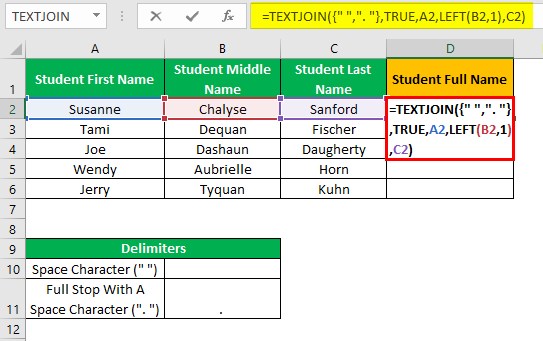
Step 2: Press Enter to view the TEXTJOIN() output.

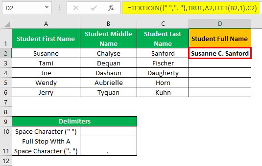
Step 3: Using the Excel fill handle, update the formula in the remaining target cells.

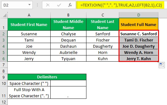
Let us check the cell D6 formula to understand its logic.

Firstly, we supply the delimiter argument value as an array of delimiters, a space character and a full stop followed by a space character. Next, we must ignore empty cells. So, the second argument, ignore_empty, is TRUE. After that, we must concatenate the first name, the first letter of the middle name, and then the last name. So, we supply the cell reference to the first name, Excel LEFT function, to display the middle name’s first letter and the cell reference to the last name as the text1, text2, and text3 arguments values.

Thus, the function inserts the first delimiter specified in the array between the first two text strings and the second between the second and third text strings. So, we get the students’ full names in the required format.

Furthermore, if we have more text strings to join, the two cited delimiters will appear alternatively in the same order between the remaining text strings.

Example #2

We shall see the steps to combine text strings with line breaks using the TEXTJOIN Excel function.

The following dataset contains employee names and their department and floor number details.

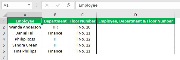
The requirement is to join the three text strings in each row, with each string starting in a new line. Assume we must display the concatenated text in column D.

Then, we can use the TEXTJOIN Excel function with CHAR(10) as the delimiter argument value. The reason to use CHAR(10) is that 10 is the linefeed character, and the CHAR(10) inserts the required line break.

Step 1: Choose cell D2, enter the TEXTJOIN(), and press Enter.

=TEXTJOIN(CHAR(10),TRUE,A2:C2)

Next, choose cell D2 and select Home - Wrap Text to view the concatenated text, with the three text strings starting in a new line or a line break in between.

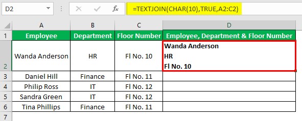
Step 2: Using the fill handle, update the formula in the remaining target cells.

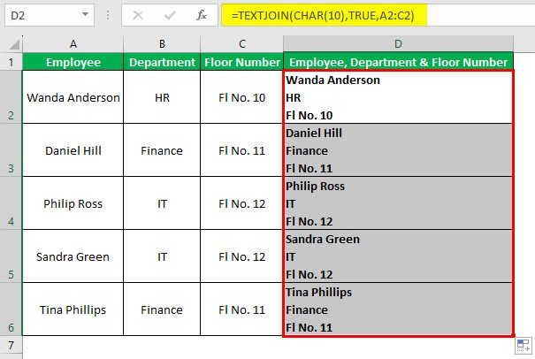
Let us check the cell D6 formula to understand how it works.

The TEXTJOIN() accepts the CHAR(10) and TRUE as the delimiter and ignore_empty argument values. Next, it accepts the cell range A6:C6, containing the text strings to merge, as the text1 argument value.

So, the function joins the three text strings, with a line break inserted between them, leading to the merged text showing the three values in new lines on enabling Excel Wrap Text.

On the other hand, consider that row 6 data is missing the department. Then, the function will ignore the empty cell and join the cells A6 and C6 text strings, with the line break in between, and the output will be as depicted below:

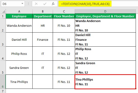
However, if the ignore_empty argument value is FALSE, then the TEXTJOIN() includes the empty cell B6 in the concatenated text in the target cell.

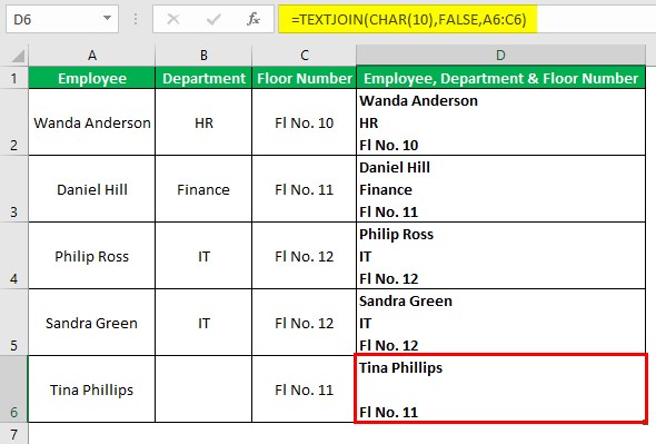
The output shows the first text string, the line break, the empty second string, the line break, and the third text string merged to give the required concatenated text.

Example #3

We can use the TEXTJOIN Excel function with conditions and formatting.

For example, the following image shows a dataset containing the monthly sales generated by sales representatives at a firm from January to March.

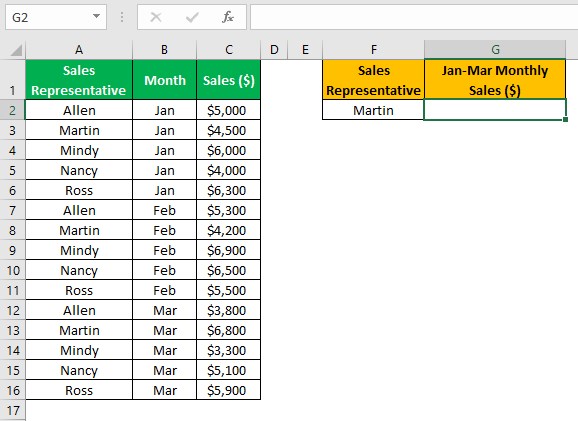
The aim is to list the sales figures of the sales representative, cited in cell F2, based on the source dataset. Further, the sales figures must be separated by a comma followed by a space character and have the same currency format as the column C data range C2:C16. Assume the target cell is G2.

Then, we can use the TEXTJOIN Excel function with the Excel IF function and TEXT excel function to achieve the required data in the desired format in the target cell.

Step 1: Choose cell G2 and enter the TEXTJOIN().

=TEXTJOIN(", ",TRUE,IF($A$2:$A$16=F2,TEXT($C$2:$C$16,"$#,##0_);($#,##0)"),""))

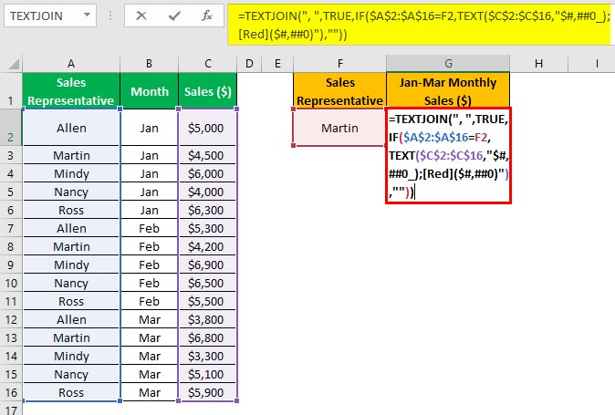
Step 2: Press Ctrl + Shift + Enter to execute the function as we would implement Excel array formulas if the Excel version is 2019. Otherwise, press Enter.

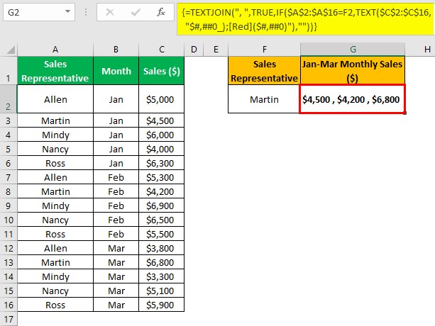
The IF statement checks each sales representative in the range A2:A16 against the target sales representative in cell F2, Martin.

If the sales representative in cell F2 matches the sales representative in column A data range, the logical condition evaluates to TRUE. Otherwise, the logical condition evaluates to FALSE. Thus, the IF() condition is an array of TRUEs and FALSEs. Hence, the formula returns an array of sales figures from column C and empty strings ("") for the TRUE and FALSE values, respectively.

Next, the array becomes the text1 argument value in the TEXTJOIN function. Further, the delimiter argument value is a comma followed by a space character, and the ignore_empty argument value is TRUE. So, the function joins the array elements with the specified delimiter in between while ignoring the empty text string elements.

Thus, we get the required sales representative’s three months of sales data as a list in the target cell.

Alternative To TEXTJOIN Function In Excel

The alternatives to the TEXTJOIN Excel function are the concatenation operator (“&”), Excel CONCATENATE function, and CONCAT() in the latest Excel versions.

For example, the following dataset shows a book, its author and copies sold data.

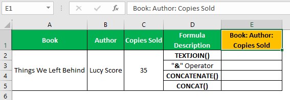
The aim is to join the three values using the formulas provided in column D to form concatenated texts in the format cited in cell E1 in the corresponding column E cells.

Step 1: Choose cell E2, enter the TEXTJOIN(), and press Enter.

=TEXTJOIN(": ",TRUE,A2:C5)

The TEXTJOIN() merges the text strings, ignoring empty cells in the specified range, with the values separated by “: ”.

Step 2: Choose cell E3, enter the concatenation operator-based formula, and press Enter.

=A2&": "&B2&": "&C2

The “&” symbol concatenates the values in cells A2, B2, and C2, and the term “: ”, in the same order as specified in the formula.

Step 3: Choose cell E4, enter the CONCATENATE(), and press Enter.

=CONCATENATE(A2,": ",B2,": ",C2)

Step 4: Choose cell E5, enter the CONCAT(), and press Enter.

=CONCAT(A2,": ",B2,": ",C2)

The CONCATENATE() and CONCAT() accept five argument values and merge the values in the same order as mentioned in the formula.

However, the noteworthy advantage of the TEXTJOIN() over the other alternatives is that we need to specify the delimiter only once in the TEXTJOIN(). But, in the case of the other formulas, we must mention the delimiters at every position where they should appear in the concatenated text.

Important Things To Note

• The TEXTJOIN Excel function is available in Excel version 2019 and above. If we try using the function in older Excel versions, the function output will be the #NAME? error value.
• If the delimiter argument value is a non-printable character or Excel does not recognize it as a text value, then the function output is the #VALUE! error value.
• If the resulting concatenated text contains more than 32,767 characters, the function returns the #VALUE! error value.

Frequently Asked Questions (FAQs)

Download Template

This article must be helpful to understand the TEXTJOIN Excel, with its formula and examples. You can download the template here to use it instantly.

Recommended Articles

This article is a guide to What Is TEXTJOIN Excel. We explain how to use the TEXTJOIN function and its alternative options with examples & points to remember. You can learn more about Excel functions from the following articles: –

• ISTEXT Excel
• TEXT Function in Excel
• Wrap Text in Excel