Table Of Contents
What is Text Function in Excel?
The TEXT excel function converts a number to a text string based on the format specified by the user. This format is supplied as an argument to the TEXT function. Since the resulting outputs are text representations of numbers, they cannot be used as is in formulas. Therefore, it is recommended to retain the original numbers and create a separate row or column for the converted numbers.
For example, the formula “=TEXT("10/2/2022","mmmm dd, yyyy")” returns February 10, 2022. Exclude the beginning and ending double quotation marks while entering this formula in Excel.
The purpose of using the TEXT function in Excel is to display a number in the desired format. Since this function also helps combine numbers with other text strings, it tends to make the output more legible. The TEXT function is particularly used when the number formats of different datasets need to be made identical.
Estimated reading time: 22 minutes
Syntax of the TEXT Function of Excel
The syntax of the TEXT function of Excel is shown in the following image:

The TEXT function of Excel accepts the following arguments:
- Value: This is the number to be converted to a text string. Apart from a number, a date, time or cell reference can also be supplied to the TEXT excel function. The cell reference can contain either a number or an output of another function which can be a number or date.
- Format_text: This is the format to be applied to the “value” argument. It is also called the format code. It is entered within double quotation marks in the TEXT formula of Excel. For instance, “0.00,” “dd/mm/yyyy,” “hh:mm:ss,” and so on are format codes.
Both the stated arguments are mandatory.
Note 1: The format code “0.00” displays a number with two decimal places. In the format code “dd/mm/yyyy,” “dd,” “mm,” and “yyyy” are the notations for days (in two digits), months (in two digits), and years (in four digits) respectively.
Likewise, “hh,” “mm,” and “ss” are the notations for hours (in two digits), minutes (in two digits), and seconds (in two digits) respectively.
For the meaning of the different date formats, refer to the heading “date formats of Excel” given after example #4 of this article.
Note 2: The TEXT function is categorized as a Text/String function of Excel. The TEXT function is available in all versions of Excel.
TEXT Function in Excel Explained in Video
How to Use the TEXT Function in Excel?
Let us consider some examples to understand the working of the TEXT function in Excel.
Example #1–Prefix the Text Strings to the Newly Formatted Date Values
The following table shows the names of five children along with the dates they were born on. The dates are currently in the format m/d/yyyy. Consider the two columns and six rows of the table as columns A and B and rows 1 to 6 of Excel.
We want to perform the following tasks:
- Join the name and date of birth of row 2 by using the ampersand operator. There should not be any space between the joined values.
- Convert each date to the format “dd mmm, yyyy.” Prefix the child’s name and the string “was born on” to each date.
- Show the output when the date of row 2 is in the format “d mmm, yyyy.” Let the prefixes of the preceding point stay as it is.
- Show the date formats “dd mmm, yyyy” (in cell C2) and “d mmm, yyyy” (in cell C6) in a single column.
Explain the outputs obtained in the second and fourth bullet points. Use the TEXT function of Excel.
| Name of Kid | Date of Birth |
|---|---|
| John | 12/8/2015 |
| Patricia | 1/12/2014 |
| Ram | 3/11/2016 |
| Anita | 11/11/2017 |
| Davis | 5/6/2014 |
The steps to perform the given tasks by using the TEXT function of Excel are listed as follows:
Step 1: Enter the following formula in cell C2. Exclude the beginning and ending double quotation marks while entering the given formula.
“=A2&“”&B2”
This formula (shown in the image of step 2) joins the values of cells A2 and B2 without any spaces in-between.
Note: The ampersand operator (&) helps join the values of two or more cells. It is called the concatenation operator and is used as an alternative to the CONCATENATE function of Excel. There is no limit on the number of cell values that the ampersand can join.
Step 2: Press the “Enter” key. The output appears in cell C2, as shown in the following image.
Notice that Excel has joined the values of cells A2 and B2 without any spaces in-between. However, the output is not in a readable format. The reason is that the date (12/8/2015) has been converted to a sequential number. The number 42346 represents the date December 8, 2015.
Note: A date is stored in Excel as a sequential or a serial number. This is because a serial number makes it easy to perform calculations. To view the serial number of a date, refer to the “note” preceding step 3 of example #2.

Step 3: To apply the format “dd mmm, yyyy” and insert the stated prefixes, enter the following formula in cell C2.
“=A2&" was born on "&TEXT(B2,"dd mmm, yyyy")”
Press the “Enter” key. Then, drag the formula of cell C2 till cell C6 by using the fill handle. The outputs are displayed in the following image.

Explanation of the outputs: In column C of the preceding image, the child’s name (in column A) and the text string (was born on) have been prefixed to each date of column B. Since the date is in a suitable format, the output is readable now.
The joined values (outputs) of column C are in the form of statements that are easier to understand than the single values of columns A and B.
Notice that, to insert spaces as the separators in the output, we have inserted spaces at the relevant places in the formula of step 1. Moreover, a comma has also been inserted after the notation of months (mmm). This comma can be seen in each date of the output (in column C).
Step 4: To see the output when the date format is “d mmm, yyyy” and the prefixes are in place, enter the following formula in cell C2.
=A2&" was born on "&TEXT(B2,"d mmm, yyyy")
Press the “Enter” key. The output appears in cell C2, as shown in the following image.
Notice that the leading zero before the date 8 Dec, 2015 (in cell C2) has disappeared. This zero was there in cell C2 of the preceding image. It has disappeared because, in the current format code, the number of days is represented by a single “d.”
A single “d” omits the leading zeros when the number of days is in a single digit.

Step 5: The outputs obtained after applying different date formats in the same column (column C) are shown in the following image.

Explanation of the outputs: Notice that in the preceding image, the date of cell C2 is in the format “d mmm, yyyy” while that of cell C6 is in the format “dd mmm, yyyy.” The only difference between these two date formats is in the number of days. The leading zero is absent in cell C2 and present in cell C6.
Hence, with the TEXT function of Excel, one can have different date formats in different cells of the same column. Remember that a format code changes only the appearance of a value; it does not change the value itself. One can create a format code depending on the requirement.
Example #2–Join the Newly Formatted Time and Date Values
The following table shows the times and dates in two separate columns. Consider these columns as columns A and B of Excel. We want to perform the following tasks:
- Join (concatenate) each time value with the respective date. Use the ampersand operator (&) and ensure that there is no space between the two values.
- Show how to copy the formats “h:mm:ss am/pm” and “m/d/yyyy” from the “format cells” window. Convert each time to the former and date to the latter format.
- Join the converted time and date values with the ampersand operator (&). Ensure that there is a space between the two values.
- Show the output when the date format is not enclosed within double quotation marks.
Explain the outputs obtained in the first and third bullet points. Use the TEXT function of Excel for the given tasks.
| Time | Date |
|---|---|
| 7:00:00 AM | 6/19/2018 |
| 7:15:00 AM | 6/19/2018 |
| 7:30:00 AM | 6/19/2018 |
| 7:45:00 AM | 6/19/2018 |
| 8:00:00 AM | 6/19/2018 |
| 8:15:00 AM | 6/19/2018 |
| 8:30:00 AM | 6/19/2018 |
| 8:45:00 AM | 6/19/2018 |
The steps to perform the given tasks by using the TEXT function of Excel are listed as follows:
Step 1: Enter the following formula (without the beginning and ending double quotation marks) in cell C2.
“=A2&“”&B2”
This formula is shown in the image of step 2. It joins the values of cells A2 and B2 without a space in-between.
Step 2: Press the “Enter” key. Then, drag the formula of cell C2 till cell C9 by using the fill handle. The fill handle is displayed at the bottom-right side of cell C2.
The outputs are shown in the following image.
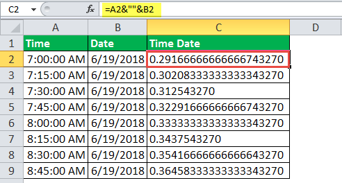
Explanation of the outputs: In column C, the number 43270 (at the end) is the same throughout the range C2:C9. This is the serial number for the date June 19, 2018. The entire decimal number preceding this serial number is the time. So, the decimal number 0.2916667 (in cell C2) represents the time 7:00:00 am.
The outputs obtained in column C of the preceding image are not readable. The reason is that Excel has converted the times (of column A) to decimal numbers and dates (of column B) to sequential numbers. Moreover, joining the decimals with sequential numbers has made the outputs more complicated.
To be able to read the output, it needs to be converted to the relevant format codes. This conversion is shown further in this example.
Note: Excel stores dates as sequential (or serial) numbers and times as decimal numbers. Excel considers a time value as a part of a day. To view the number representing the date, perform the following actions:
- Select any cell of the range B2:B9.
- Press the keys “Ctrl+1” together. The “format cells” window opens.
- Select “general” under “category” in the “number” tab.
The serial number can be seen under “sample.” Click “cancel” to close the “format cells” window or “Ok” to change the date to a serial number.
Likewise, the decimal number representing the time can also be seen by selecting any cell of the range A2:A9 and following actions “b” and “c” listed above.
Step 3: To convert the time and date values to a readable format, let us first copy the format codes from the “format cells” window. So, select cell C2 and press the keys “Ctrl+1” together.
The “format cells” window opens, as shown in the following image. From the “number” tab, select “custom” under “category. Excel provides a list of formats under “type.”
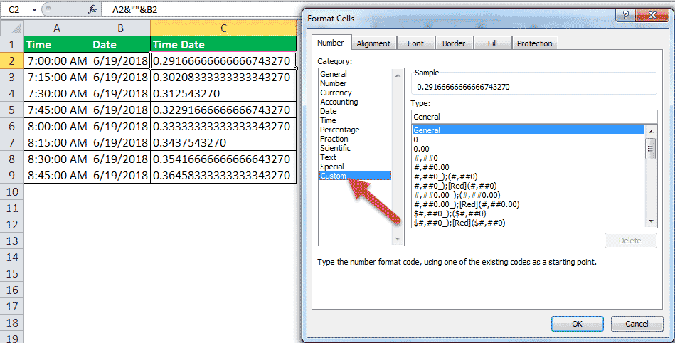
Step 4: Scroll down the list of formats given under “type.” Copy the format “h:mm:ss am/pm.” To copy, just select the format code and press the keys “Ctrl+C.”
The format code is shown in the following image. Once the format has been copied, close the “format cells” window.

Step 5: Copy the format code “m/d/yyyy” for converting the date values. This format code is also available under “type,” as shown in the following image.
Close the “format cells” window after copying the mentioned format code.

Step 6: To apply the new formats to the time and date values and join the resulting values, enter the following formula in cell C2.
“=TEXT(A2,"h:MM:SS AM/PM")&" "&TEXT(B2,"m/d/yyyy")”
This formula is shown in the image of step 7. If the format codes have been copied in the preceding steps, they can be pasted at the relevant places in the formula by pressing the shortcut “Ctrl+V.”
According to this formula, the time and date values of cells A2 and B2 are formatted as per the codes "h:MM:SS AM/PM" and "m/d/yyyy" respectively. The formatted (or converted) values are then joined with the ampersand operator.
Notice that in the formula, a space has also been entered within a pair of double quotation marks (like &“ ”&). This space will be inserted in the output at exactly that place where it has been entered in the formula.
Step 7: Press the “Enter” key after entering the TEXT formula. Drag the formula of cell C2 till cell C9.
The outputs are shown in the following image.
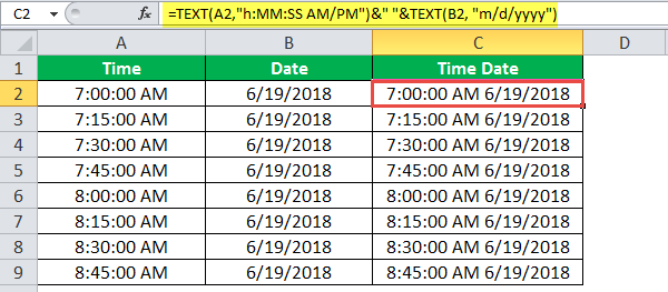
Explanation of the outputs: The time and date values of columns A and B have been converted to the relevant formats in column C. The time values display the hours (h) in a single digit, minutes (mm) in two digits, and seconds (ss) also in two digits. Since all the time values belong to the period before noon, they display “am” at the end.
Likewise, the dates display the months (m) in a single digit, days (d) in a single digit, and years (yyyy) in four digits.
Notice that there is a space between the two joined values in column C. Even though we copied the code “h:mm:ss am/pm” (in step 4) and pasted “h:MM:SS AM/PM” (in step 6), we obtained the correct outputs in column C (in step 7). This is because the format codes are not case-sensitive, implying that “mm” is treated the same as “MM.”
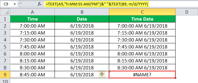
Step 8: To see what happens when the format code for date is entered without the double quotation marks, type the following formula in cell C9.
“=TEXT(A2,"h:MM:SS AM/PM")&" "&TEXT(B2,m/d/YYYY)”
Press the “Enter” key. Excel returns the “#NAME?” error, as shown in the following image. Therefore, for the TEXT excel function to work, the format code should necessarily be enclosed within double quotation marks.
Example #3–Extract a Mobile Number from its Scientific Notation
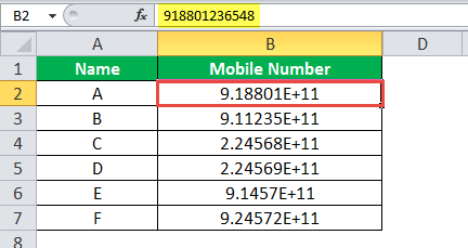
There are two images titled “image 1” and “image 2.” The following information is given:
- Image 1 shows a number having eleven 9s in cell B2. When 1 is added to this number, its digits increase to 12. Excel displays the resulting 12-digit number (in cell B3) in a scientific notation.
- Image 2 shows the names of some people (in column A) and their random mobile numbers in a scientific notation (in column B). The formula bar shows the mobile number of person A. Each mobile number consists of twelve digits, which includes a 2-digit country code at the beginning.
Note that a scientific notation (or scientific format) often displays very large or very small numbers in a contracted form. We want to perform the following tasks:
- Display the entire 12-digit mobile number without any spaces in-between.
- Separate the country code from the rest of the number with the help of a hyphen.
Use the TEXT function of Excel for the given tasks.
Image 1
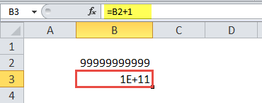
Image 2
The steps to perform the given tasks by using the TEXT function of Excel are listed as follows:
Step 1: Enter the following formula in cell D2.
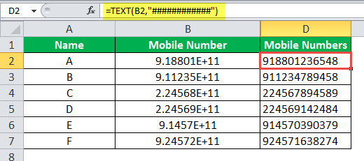
“=TEXT(B2,"############")”
This formula is shown in the formula bar of the succeeding image. Notice that there are 12 hashes in the formula, which represent the 12 digits of a mobile number.
Step 2: Press the “Enter” key. The output appears in cell D2. To obtain the outputs for the entire column D, drag the formula of cell D2 to cell D7. Use the fill handle of cell D2 (displayed at the bottom-right corner) for dragging.
The outputs of column D are shown in the succeeding image.
Note: The output is displayed (in column D) only when one enters a mobile number as an input (in column B) which is converted automatically (or manually) to a scientific format of Excel. In case, a scientific format is typed manually in column B; it cannot be converted to a mobile number of column D.
Step 3: To separate the country codes from the rest of the number by using a hyphen, enter the following formula in cell D2.
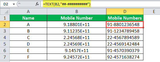
“=TEXT(B2,“##-##########”)”
Press the “Enter” key. Next, drag the formula of cell D2 till cell D7 with the help of the fill handle. The formula of cell D2 and the outputs are shown in the following image.
Notice that in the formula, the hyphen is placed exactly where it is required in the output. Since only the first two digits of each mobile number are to be separated, the hyphen is placed after two hashes of the formula.
Example #4–Prefix a Text String to the Initially Formatted Monetary Value
There are two images titled “image 1” and “image 2.” The following information is given:
- Image 1 shows the gross profit, expenses, and net profit of an organization. All these numbers are in dollars.
- Image 2 shows how the net profit has been computed. To calculate the net profit, the expenses have been subtracted from the gross profit.
We want to perform the following tasks:
- Show the output when the string “the net profit is” is prefixed to the amount of net profit. Use the ampersand operator for this purpose.
- Prefix the string “the net profit is” to the amount of net profit by using the ampersand. Ensure that in the output, the amount of net profit displays the dollar sign ($) and the comma at the correct places (like $52,291). Use the TEXT function of Excel for this purpose.
Explain the output obtained at the end.
Image 1

Image 2
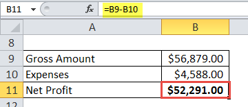
The steps to perform the given tasks are listed as follows:
Step 1: Enter the following formula in cell A13.
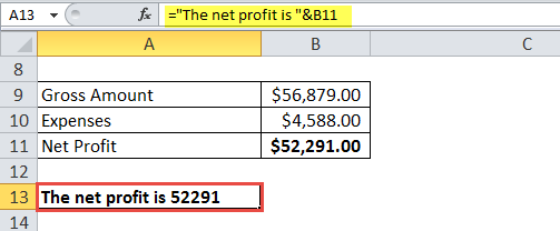
“="The net profit is "&B11”
Exclude the beginning and ending double quotation marks of the formula while entering it in Excel. This formula is shown in the image of step 2.
The given formula prefixes the string “the net profit is” to the value of cell B11. The ampersand helps join the stated string to the amount of net profit (in cell B11).
Step 2: Press the “Enter” key. The output appears in cell A13, as shown in the following image.
Notice that the dollar sign and the comma of the net profit amount (shown in cell B11) have been omitted in the output. Though the string “the net profit is” has been correctly prefixed. The spaces have also been inserted at the right places in cell A13.
Step 3: To retain the dollar sign and the comma of the amount, enter the following formula in cell A13.
“="The net profit is " &TEXT(B11,"$#,##0.00")”
Press the “Enter” key. The formula and the output are shown in cell A13 of the following image.
Notice that by mistake, a space has been inserted before the ampersand in the formula. However, even then, the correct output has been obtained in cell A13.
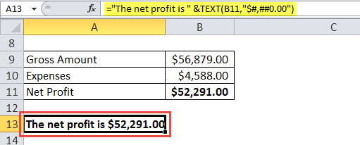
Explanation of the output: This time, the amount of net profit has been properly written (including the dollar sign and the comma) in cell A13. The reason is that the amount of net profit has been converted to the appropriate format in addition to being prefixed by a text string.
So, with the TEXT function of Excel, one can join a number with any string and, at the same time, retain the initial formatting of the number.
Date Formats of Excel
The different format codes for dates have been described as follows:


