SUMPRODUCT With Multiple Criteria

SUMPRODUCT with multiple criteria in Excel helps compare the arrays with numerous criteria.

The format for SUMPRODUCT with multiple criteria in Excel will remain the same as the SUMPRODUCT formula. The only difference is that it will have multiple criteria for two or more ranges and then add up those products.

For example, consider the below table showing sample with expected and actual sales. Now, assume that we have to find the sample with less sales than the expected sales.

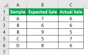
The steps are:

Step 1: Firstly, we should insert the SUMPRODUCT formula in the desired cell.

Step 2: The formula is =SUMPRODUCT((C2:C6<B2:B6)*(A2:A6="B"))

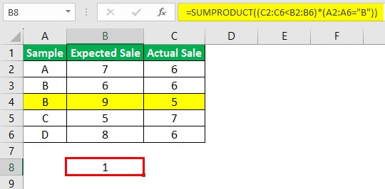
Likewise, we can use the SUMPRODUCT formula with multiple criteria in Excel.

• SUMPRODUCT with multiple criteria is a method used to obtain results using SUMPRODUCT formula with criterias.
• We can use this function in place of formulas like SUMIF, COUNTIF, etc.
• Also, we can use it to create a complex formula that sums up the arrays’ rows and columns.
• Similarly, users can use SUMPRODUCT function in Excel with logical operators like AND, OR, & both.
• The wild card characters like an asterisk (*) and question mark (?) are not valid using the SUMPRODUCT formula.

1. We can use it in place of formulas like SUMIF, COUNTIF, etc.
2. We can use it to create a complex formula that sums up the arrays’ rows and columns.
3. We can use it with logical operators like AND, OR, & both.

Let us learn this SUMPRODUCT formula with the help of following examples.

Example #1

Let us assume we have a list of company products in the second column. The third column is for the planned count of products to be sold, and the actual sales happened in column fourth. Now, the company wants to determine how many platinum products sold have made fewer sales than the planned count.

Example #2

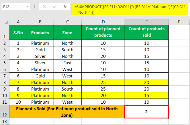
Let us assume we have a list of company products in the second column, zone in the third column, and fourth for the planned count of products to be sold. The actual sales that happened are in the fifth column. The company wants to determine how many platinum products sold in the north zone have made less than the planned count.

• Data for the above case is shown below:

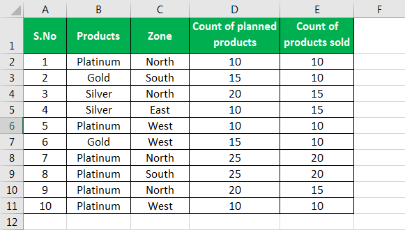
• In this case, we have two conditions: Firstly, to find the count of the number of products that are less than the planned count. Secondly, that count should be of a platinum product only. Thirdly, they should sell that product in the “North” zone.

Now, we will use the SUMPRODUCT formula in excel to calculate the count with multiple criteria.

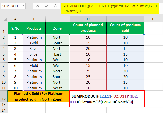
• The final count of the number of sold products which are less than planned, that too product should be platinum which lies in “North” zone is shown below:

Example #3

Let us assume that student Andy has completed his exams and has a list of expected and obtained marks in various subjects. Column A shows the subject and columns B and C shows the expected and obtained marks.

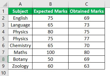
• In this case, we have two conditions: Firstly, to find the count of subjects where he has obtained less than the expected marks.

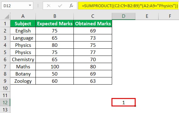
Now, we will use the SUMPRODUCT formula in excel to calculate the count with multiple criteria.

We can see the result as shown in the below image.

• There should be the same number of rows and columns in all the SUMPRODUCT formulas. Otherwise, it will return an error.
• The SUMPRODUCT formula treats all the non-numeric values as zero.
• Without using a double negative sign or multiple the formula with one, the SUMPRODUCT formula will return an error.

This article is a guide to SUMPRODUCT with Multiple Criteria in Excel. Here, we discuss using the SUMPRODUCT function with multiple criteria in Excel, examples, and a downloadable Excel template. You may also look at these useful functions in Excel: -

• SUMIF With VLOOKUP
• SUMIF Between Two Dates in Excel
• VLOOKUP with SUM