SUMIFS In Excel

The SUMIFS in Excel is an enhanced function of the SUMIF formula in Excel that enables us to sum up any range of data by matching several criteria. In the SUMIFS function in Excel, we can enter up to 127 criteria_ranges and criteria pairs.

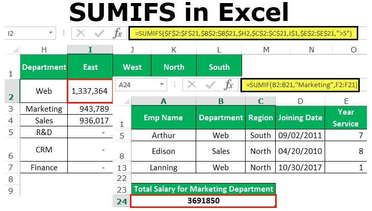
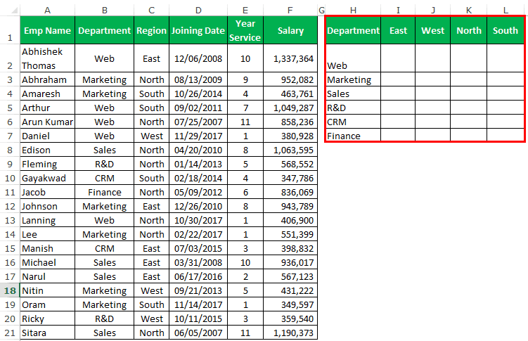
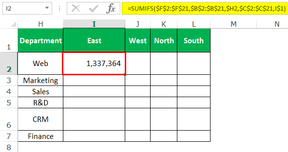
For example, in the given dataset, we can find the sum of all the values that fall under the “Web” department of the “East” region, as shown in cell I2.

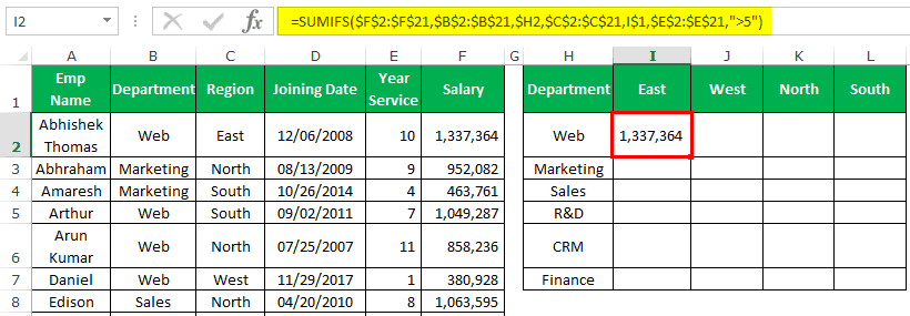
The output is derived with multiple criteria, such as the set department in a particular region. The values are retrieved first, and then the total is calculated.

The syntax of the SUMIFS Formula is,

The arguments of the SUMIFS Formula are,

• sum_range: The cells or range of cells that you want to SUM. For example, the A1:A20 range.
• criteria_range1: The column which includes the first criteria values.
• criteria1: The first condition to retrieve the value from.
• criteria_range2: The second column, which includes the second criteria values.
• criteria2:  The second condition to retrieve the value from.

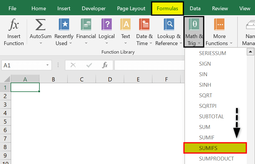
We can insert the SUMIFS Function in Excel in multiple ways. One way is by inserting it from the “Function Library”, as follows:

First, keep the dataset ready → select the “Formulas” tab → go to the “Function Library” group → click the “Math & Trig” option drop-down → select the “SUMIFS” function as shown below.

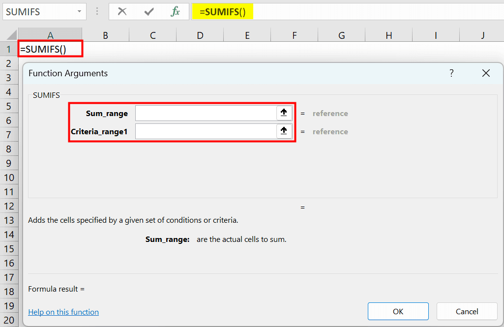
The “Function Arguments” window opens. Enter the cell range in the “Sum_range” and the “Criteria_range1” fields, and click “OK”, as shown below.

We will consider some examples for the SUMIFS Function in Excel.

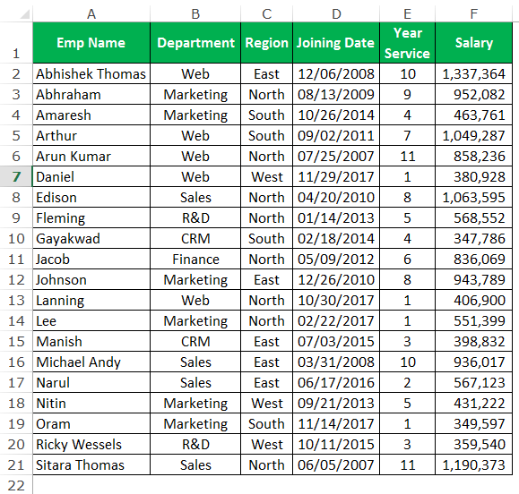
The table below includes the employment history with the employee names, the department they belong to, years of service in the company, and their salaries.

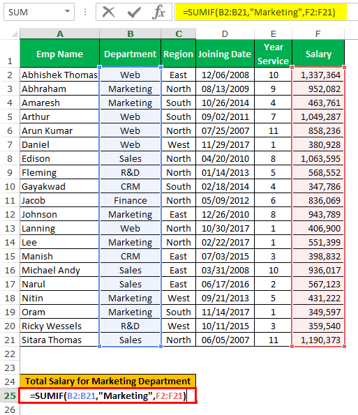
Now, first, look into the SUMIF example. Using SUMIF, the function calculates the total salary for the Marketing department.

It gives the output as shown below:

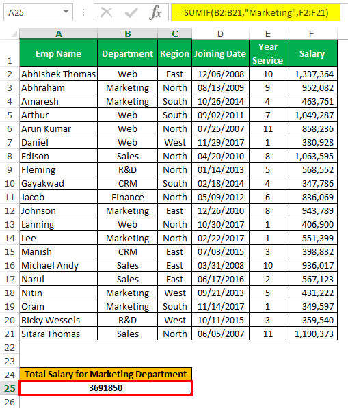
The above image shows the total salary for the marketing department. The SUMIF function can take only one set of criteria.

What if you want to sum up the total salary for the marketing department in the northern region? In multiple criteria-based situations, we can use the Excel SUMIFS function to calculate the salary.

To calculate the total salary for each department across four different regions, let’s take our first criterion as the department and the second criterion as the region.

The steps to calculate the total salary are,

1. Create a table that includes departments and regions by removing all the duplicate values. Your table should look like the one below.

2. Apply the SUMIFS function in the table. Open the SUMIFS function in Excel.

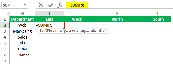
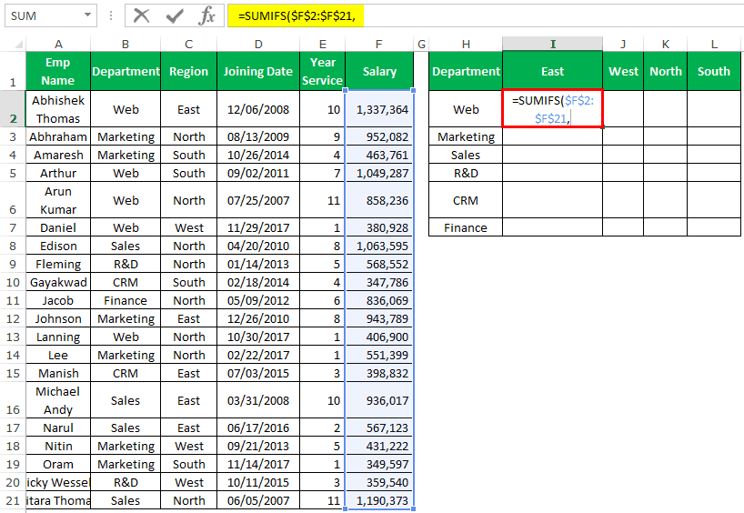
3. Select the sum_range as F2 to F21.

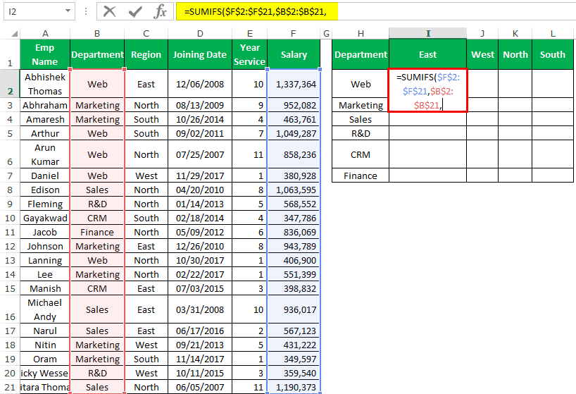
4. Select the B2 to B21 as the “criteria_range1.”

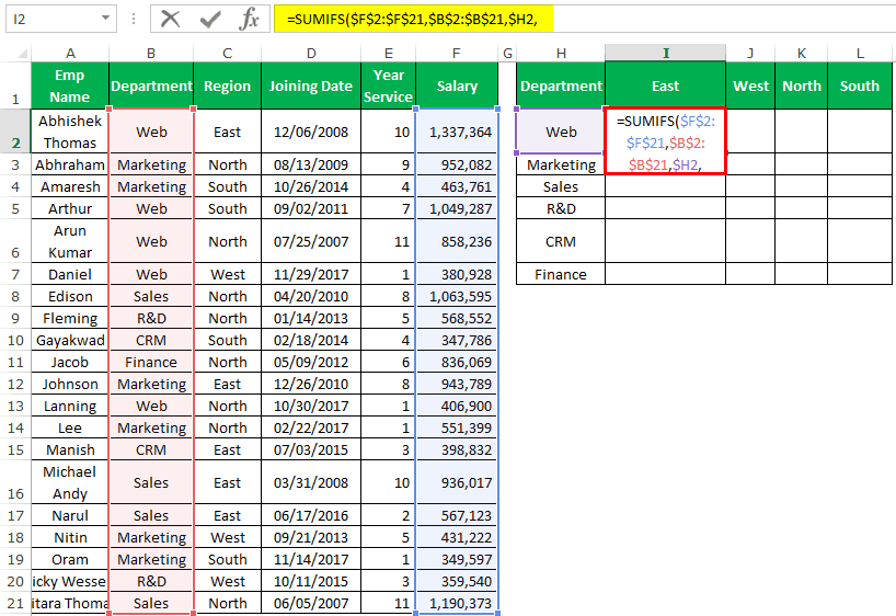
5. The “criteria” will be the “Department.” So, select the cell H2 and lock only the column.

6. The “criteria_range2” will be C2 to C21.

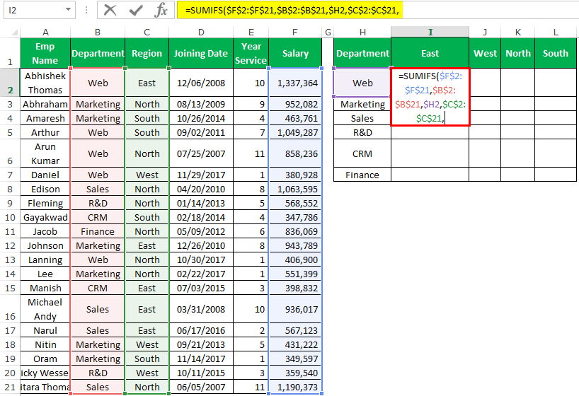
7. For this “criteria_range”, the criteria is “East,” so select the I1 cell as the reference and lock the only row here.

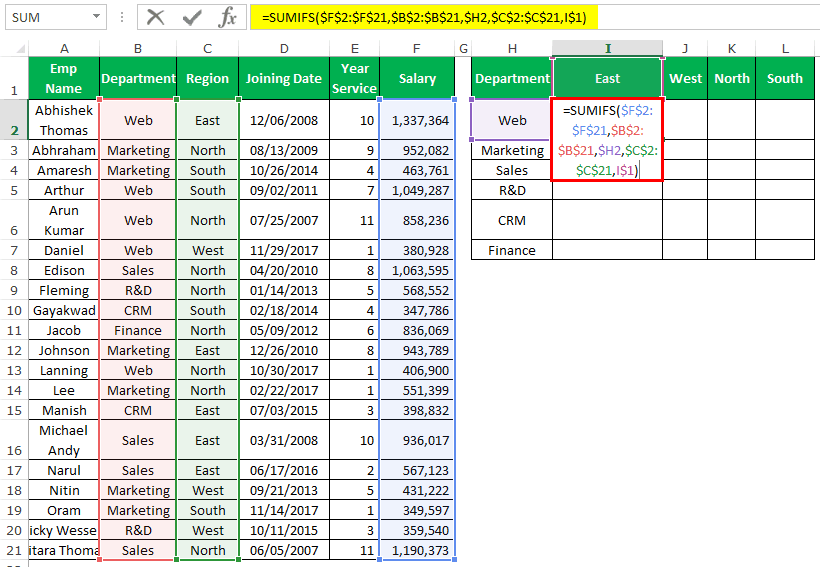
8. We now have value for the department “Web” and the region “East.”

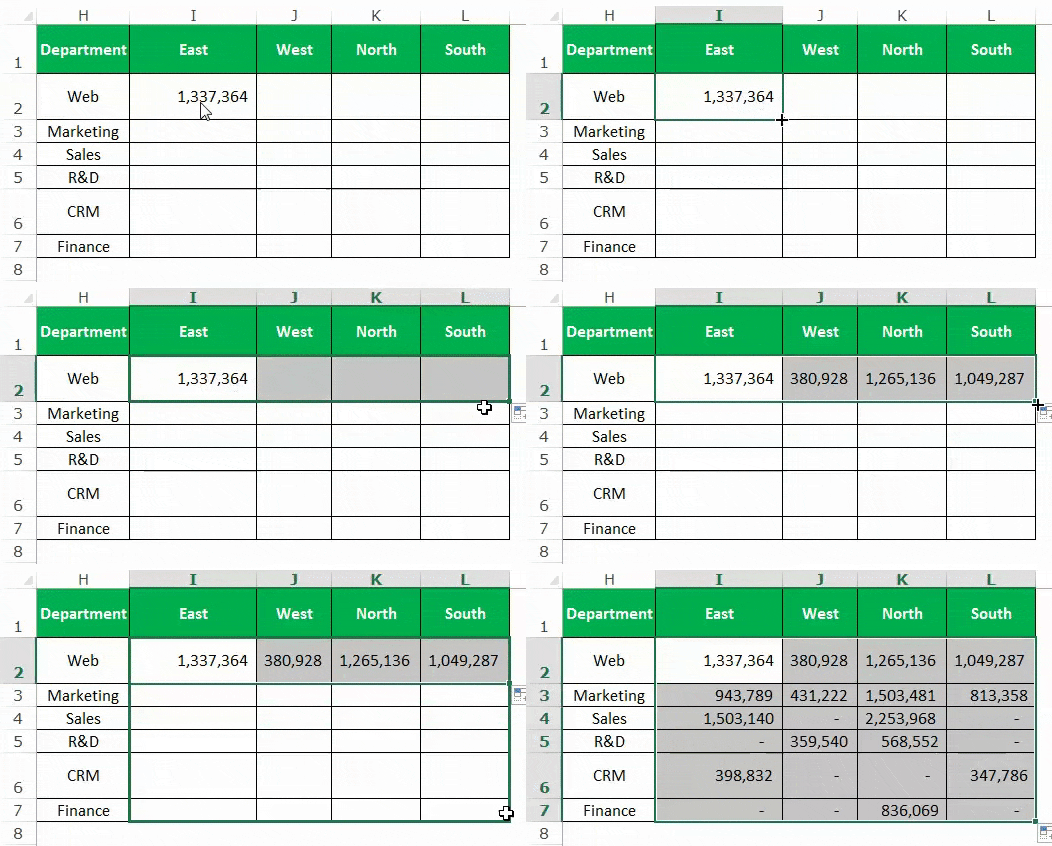
9. Now, drag the formula to the remaining cells to have the result in all the cells.

Now, look at the detailed explanation of the formula part by part.

• Yellow Part: Yellow color is the first part of the formula that asks which column you want to sum. Our required column to sum is the salary column from F2:F21. We have locked this range (absolute reference) because this range should be standard when we copy-paste the formula to other cells.
• Green Part: It is the second part of the formula. We are considering this as our first criteria range. The first criteria we need to apply is a department column, and the department column range is B2:B21. We have locked this range (absolute reference) because this range should be standard when we copy-paste the formula to other cells.
• Grey Part: It is the extension of the Green Part. We are giving the criterion to the criteria range we have selected in the Green Part. Our criterion is in the cells from A23:A29. One interesting thing is we have locked only the column part ($H2) because when we move to the right side. The column should be standard, and when we are moving down, the row should change. For example, if we copy-paste the formula to the next cell, we should change $A23 to $A24.
• Pink Part: It is the third part of the formula. We are considering this as our second criteria range. The second criteria we must apply is the region column, and the region column range is C2:C21. We have locked this range (absolute reference) because this range should be standard when we copy-paste the formula to other cells.
• Blue Part:  It is the extension of the Pink Part. We are giving the criterion to the criteria range we have selected in the Pink Part. Similar to the Grey Part of the formula.

In the previous example, we have seen two criteria in one SUMIFS Excel example. Assume you want to calculate the total salary for each department across four different regions if the year of service is greater than 5 years. Here, our first criterion is a department, the second criterion is the region, and the third criterion is a year of service.

The steps to calculate the total salary are,

It is the same as the above example.

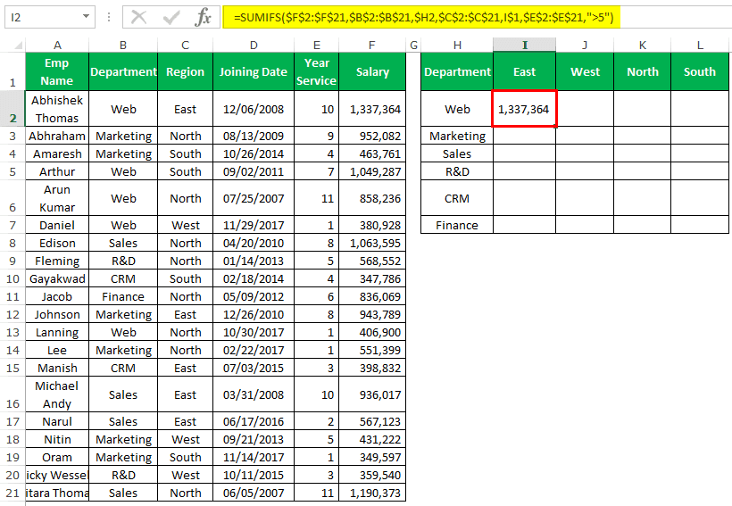
We need to continue the formula after two criteria.

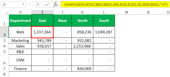
Now, look at the detailed explanation of the formula part by part.

We have already discussed the Yellow Part, Green Part, Grey Part, Pink Part, and Blue Part. The only thing we have added here is Years’ Service as our third criteria column, and “>5” is the criteria we are giving.

Since we need to add the salary if the years of service are greater than 5 years, we have used the operator symbol (>). In the SUMIFS function, we can use an operator symbol to get the job done.

Below are some of the operator symbol examples.

• “>5”: Greater than 5 years.
• “>=5”: Greater than or equal to 5 years.
•  “=5”: Equal to 5 years.
• “<5”: Less than 5 years.
• “<=5”: Less than or equal to 5 years.
• “<>”: It is a non-blank cell.

• We can apply the SUMIFS function in Excel to 127 criteria ranges. All the ranges should be of the same length. For example, Excel will throw an error if the sum_range is C1:C10 and the criteria_range is A1:A9.
• The numerical values need not be enclosed in double-quotes. However, you need to use double quotes if we use numerical values with operators.