SUMIF With VLOOKUP

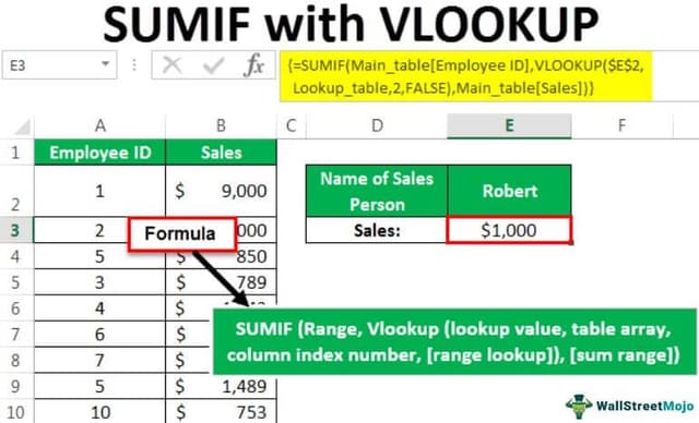
The SUMIF with VLOOKUP is a combination of two different conditional functions. The SUMIF function is used to sum the cells based on some condition which takes arguments of the range with the data and then the criteria or the condition and cells to add. Instead of the criteria, we can use the VLOOKUP as the criteria when there is a large amount of data available in multiple columns.

For example, suppose we have a dataset and want to sum values according to conditions. Still, you also have to look up another table to get the correct criteria value. In such a scenario, we can combine the SUMIF and VLOOKUP functions in one formula.

The SUMIF is a function presented in Excel from the 2007 version presented in Excel to sum the various values that match the criteria. The VLOOKUP function is one of the best formulas to gather data from other tables. When multiple conditions and columns exist, SUMIF(VLOOKUP) is used to perform numerous calculations on the Excel sheet. The disadvantage of the SUMIF function returning the only number is overcome using VLOOKUP. The VLOOKUP function helps to return any data from a table based on the matched criteria.

SUMIF Function: It is a Math and Trigonometry function to sum the values when the established condition is "TRUE." The sum value is obtained based on only one criterion.

When we deal with the SUMIF function in Excel, the following formula is used:

• Range: It is the range of the cells used to assess the established criteria.
• Criteria: It is the condition to sum the values. It may be a cell reference, number, and another Excel function. For example, when we want to combine SUMIF and VLOOKUP, it will enter the VLOOKUP function in the place of the criteria.
• Sum_range: The range of cells specified to sum the numerical values.

Now, the formula is modified to

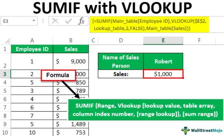
Formula = SUMIF (Range, Vlookup (lookup_value, table_array, column _index _number, ), )

• Lookup_value: It specifies the value to be searched in a table. It may be a reference or value.
• Table_array: It is the range of the table containing two or more two columns.
• Column_index_number: The relative index of a column specifies for returning required data from a specific column.
• : It can be 0 or 1 to specify whether it should return the exact or approximate value. But, it is optional to a user. 0 indicates an exact match, and 1 shows an approximate match.

The combined use of SUMIF(VLOOKUP) is helpful in searching data based on a single criterion. Excel uses these in many ways to perform the calculations by searching for data. These are collectively used in the business environment to perform various tasks to make good decisions. To use these functions effectively together,

First, the SUMIF function is to be entered utilizing the two methods.

First Method: The formula must type from the keyboard, as shown in the image below.

Second Method: The SUMIF function can be inserted from the "Formulas" tab as shown in the image.

After entering the SUMIF function, the formula for VLOOKUP is entered inside the SUMIF function by replacing the "Criteria" element. All the parameters of the VLOOKUP, including the lookup value, table array, index number of the column, and range lookup. These are to be enclosed in parenthesis to avoid errors with the formula. The values to be summed are included in the sum range elements of the SUMIF function. At last, "CTRL," "SHIFT," and "ENTER" keys are pressed together to facilitate the values as an array.

Example #1 - Use of sumif(vlookup) together to determine some value

This example shows how to use the SUMIF(VLOOKUP) together to find the sum of the sales in the same month in different years.

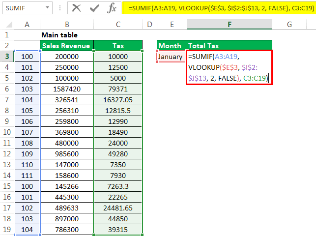
• The following data is considered for this example, as shown in the screenshot.

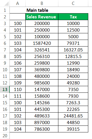
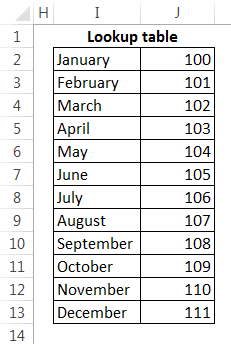
• The lookup table considered is shown as mentioned below. In addition, it included reference values for the months from January to December.

• After entering data into the main and lookup tables, the SUMIF function determines the total sales generated in other months. Here, the Lookup value considered is the month. The formula combining the SUMIF(VLOOKUP) is shown as:

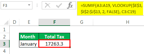
The total sales in January month are determined as 17263.3. When we change the lookup value to another month, the respective total sales are generated.

Example #2 - Determining Sum Based on Matching Criteria in Different Work Sheets

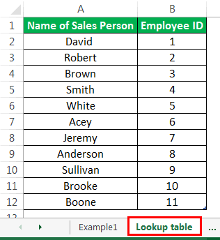
In this example, the lookup table and main table are taken in different sheets rather than a single sheet. As a result, the lookup table data is shown in the below screenshot.

The main table data is shown in the below screenshot.

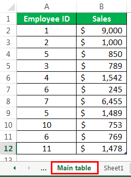
The salesperson's name is taken as a lookup value for determining the total sales, and employee IDs are used for reference purposes. The formula is entered as presented below, and few changes are observed to the formula compared to the first example.

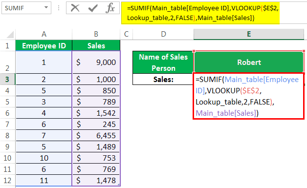
In this example, instead of selecting a lookup array, only lookup_table is mentioned. By pressing the three keys, including "CTRL," "SHIFT," and "ENTER," accurate results are produced.

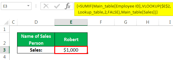
When the salesperson's name is changed to names mentioned in the lookup, the sum of sales is varied and produces a new result.

The following are the benefits of using these functions:

• We can easily extract the values from another table to perform calculations.
• Determining the sum of values presented in a range that meets the criteria mentioned in different aspects of a business.

• While using the VLOOKUP function, the column index number should not be lower than 1 to avoid errors.
• We should give indexes to the lookup table columns by indicating numbers 1, 2, 3, and so on.
• The CTRL+SHIFT+ENTER in excel should be used instead of entering the key since the VLOOKUP function is entered as an array formula.
• Defining two tables, including main and lookup, is required to extract values and determine the sum of the array values.
• The SUMIF function provides accurate results for only numerical data. It would not work for another kind of data.