SUMIF Not Blank

Publication Date :

13 Jul, 2019

Blog Author :

Edited by :

Reviewed by :

Download FREE SUMIF Not Blank In Excel Template and Follow Along!

SUMIF Not Blank Excel Template.xlsx

Table Of Contents

What Is Excel SUMIF Not Blank?

SUMIF not blank in excel is a very simple function used to find the total of a specific criteria in the data. First, we use “ “ as a criterion for a blank cell. But, to use SUMIF when only the cells are not blank as the criteria, we can use the operator “<>,” which means not equal to blank. This operator acts as the criteria for the function in summing up the cells when the criteria range is not blank.

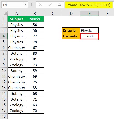
For example, consider the below table showing the highest marks obtained by students in 4 semesters. Now, assume that we have to calculate the sum of all the highest marks in semester 1.

The steps are:

Step 1: First, select the cell where we want to insert the result. So, in this example, select cell E4.

Step 2: Then, enter the arguments in the Function Arguments window.

Step 3: Click OK. We can immediately see the results in cell E4.

Likewise, we can use SUMIF not blank in Excel.

In this article, we will learn how to use SUMIF not blank and how to select the values for arguments with examples.

Key Takeaways

SUMIF not blank in Excel is a formula used to find the total based on the criteria.
The formula of SUMIF is =SUMIF(range,criteria,) where all 3 arguments are mandatory.
In Range argument, we have to select the cell range with different criterias.
Similarly, we have to select the cell specifying the criteria based on which the total sum is calculated.
Finally, sum_range is the argument where we have to select the cell range with the values.
We can simply click on Formulas - Math & Trig - SUMIF to insert the formula in Excel.

Syntax

The syntax of SUMIF is =SUMIF(range,criteria,) where all 3 arguments are mandatory.

How To Use Excel SUMIF Not Blank?

This article must be helpful to understand the Excel SUMIF Not Blank, with its formula and examples. You can download the template here to use it instantly.

SUMIF Not Blank Excel Template Download

Examples

Example #1 - SUMIF Not Blank

The below set of data contains certain blanks in the range criteria. Suppose we still want to know the total no. of passengers:

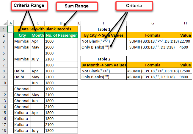
Here now, criteria range conditions completely change for both by city and month. Important to note the condition which we put here in the syntax for criteria:

<>” -> indicates the “NOT EQUAL TO” sign. It has to be in double inverted commas as the formula processes it as characters. When we use this, the formula sums up all the values that are not blanks and completely ignores the blank cells during summation.
“-> indicates “Blanks.” Double inverted commas with no characters in them signify equal to blank. When we use this, it sums up all the values containing blanks and ignores cells containing some characters/values.

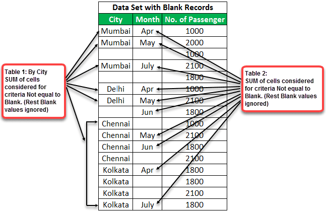
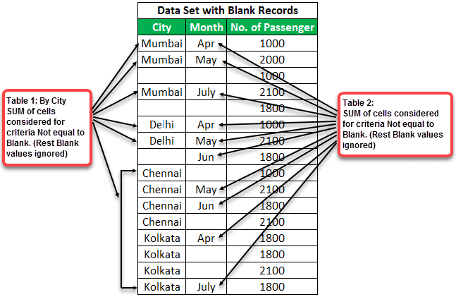
For the ease of understanding the final output of tables 1 and 2. Refer to the below explanation:

Example 2 - Using Function Argument

Let us look at the example.

Select cell F2(active cell), where we need SUMIF() value as shown below:
Click on the “Formulas” tab and select “Math & Trig.”
A dropdown appears with various mathematical functions in Excel. For example, click “SUMIF”(highlighted in red).
A dialog box appears, as shown below. The next steps would be to input corresponding respective cell references or values:

Here, we will insert the cell reference of the “City” column in “Range” input, “City name/ cell reference” in “Criteria” input, and “No. of Passenger” in “Sum_range.”
Go to the “Range” section in the dialog box, click in the blank space, select range starting from A2, and drag up to A17. Next, select all the row ranges in “City” column B. Then, go to the “Criteria” section and select the “City” cell reference, cell E2. Similarly, go to the “Sum_range” section in “Column C” and choose from C2 to C17.
Click on “OK” and see the value in cell E2.

Example 3

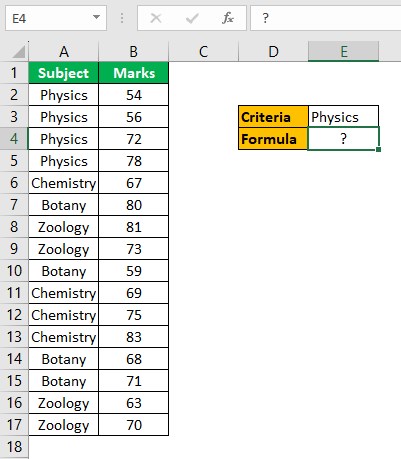
Select cell E4(active cell), where we need SUMIF() value as shown below:
Click on the “Formulas” tab and select “Math & Trig.”

SUMIF Not Blank - Example 3 - Math-Trig.jpg

A dropdown appears with various mathematical functions in Excel. For example, click “SUMIF”(highlighted in red).

SUMIF Not Blank - Example 3 - Step 3.jpg

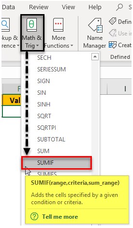
A dialog box appears, as shown below. The next steps would be to input corresponding respective cell references or values:

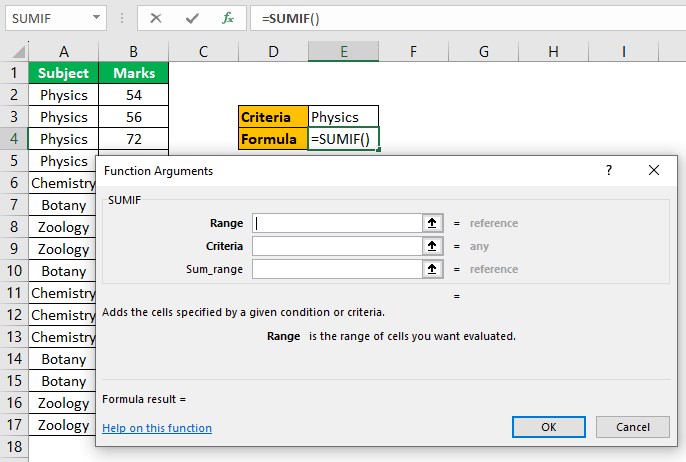
Here, we will insert the cell reference of the “Subject” column in “Range” input, “Physics” in “Criteria” input, and “Marks” in “Sum_range.”

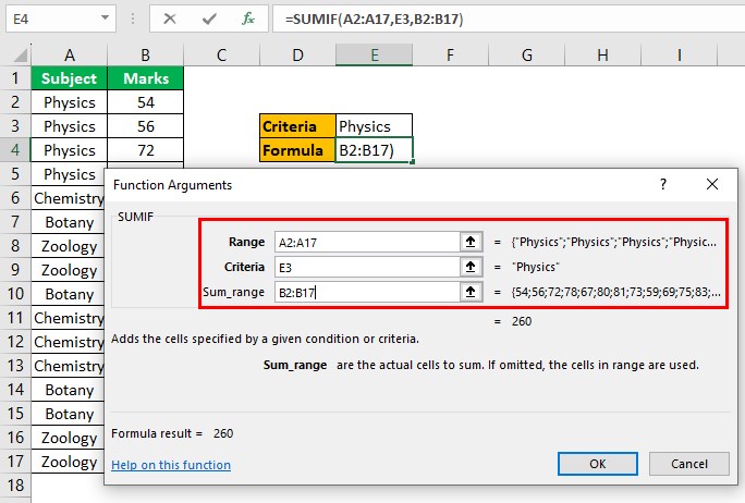
Example 3 - Step 4 - Function Argument.jpg

Click on “OK” and see the value in cell E4.

Important Things To Note

The SUMIF Not Blank has limited use unless that dataset contains blank rows in the criteria range.
We have to specify the cell range properly to obtain proper results.