SUMIF Excel Function

The SUMIF Excel function calculates the sum of a range of cells based on given criteria. The criteria can include dates, numbers, and text. For example, the formula “=SUMIF(B1:B5, “<=12”)” adds the values in the cell range B1:B5, which are less than or equal to 12.

SUMIF function is categorized under the Excel Math and Trigonometry functions. Moreover, this function works similar to the SUMIFS function. The SUMIF function uses a single criterion, whereas the SUMIFS function uses multiple criteria.

The SUMIF formula is stated as follows:

The formula accepts the following arguments:

• Range: It refers to the range of cells on which the criteria is applied.
• Criteria: It refers to the conditions that are applied to the range of cells. It determines the cells to be added from the given “sum_range.”
• Sum_range: It indicates the range of cells to be added together.

“Range” and “criteria” are the required parameters, whereas “sum_range” is an optional parameter.

Note: If “sum_range” is not specified, the SUMIF function refers to the parameter “range” as the range of cells to be added.

Let us understand the SUMIF excel function with the help of the following examples. Each example covers a different case, implemented using the SUMIF function.

Example #1

Total Amount Spent on Branded Televisions (TVs)

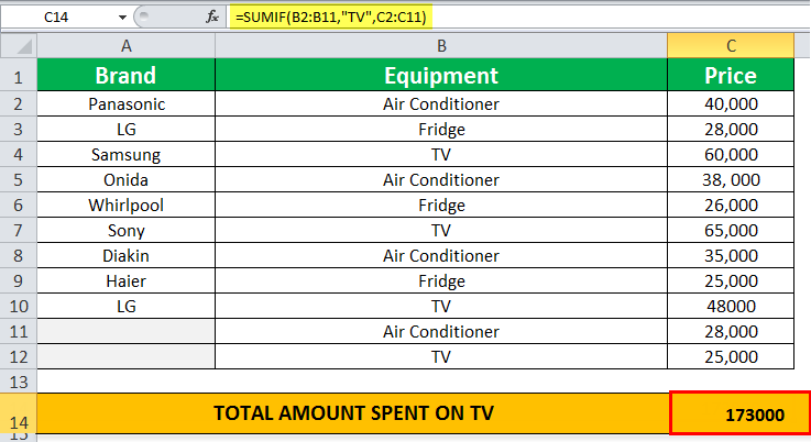
The following table shows a list of branded equipment and their prices. For some equipment, the brands are not specified.  We have to calculate the total amount spent on purchasing branded TVs using the SUMIF function. 

In the succeeding table, the cells that satisfy the given criteria are C4, C7, and C10, which shows the prices of the branded TVs. Hence, the sum of the values of cells C4, C7, and C10 is 1,73,000, shown in cell C14. This is the total amount spent on purchasing branded TVs.

The following SUMIF formula is applied to the range C2:C11:

“=SUMIF(B2:B11,“TV”,C2:C11)”

Where,

• B2:B11 refers to the range of cells on which the specific criterion is to be applied.
• “TV” refers to the condition applied to the range B2:B11.
• C2:C11 refers to the range of values to be added.

Example #2 

Sum of the Amount Spent on Non-Branded Items

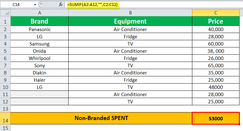
Working on the data of example #1, we want to calculate the total amount spent on purchasing non-branded items using the SUMIF function.

In the following table, the cells C11 and C12 satisfy the given criteria where no brand name is entered in the cells. Hence, the sum of the values of cells C11and C12 is 53,000, as shown in cell C14. This indicates the total amount spent on purchasing non-branded items.

The following SUMIF formula is applied to the range C2:C12:

“=SUMIF(A2:A12,“”,C2:C12)”

Where,

•  A2:A12 refers to the range of cells on which the specific criterion is to be applied.
• “” refers to the condition which checks for blank cells in the range B2:B12.
• C2:C12 is the range of values to be summed up.

Example #3

Sum of the Amount Spent on Branded Items

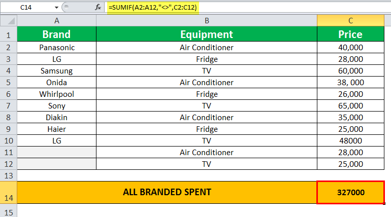
Working on the data of example #1, we want to calculate the total amount spent on branded items using the SUMIF function.

In the following table, the cells B11, B12 satisfy the given criteria with no brand names. Hence, the sum of the values of C1 to C10 is 53,000, displayed in cell C14. This is the total amount spent on purchasing branded items. The cells C11 and C12 are skipped because they are blank cells.

The following SUMIF formula is applied to the range C2:C12:

“=SUMIF(A2:A12,“<>”,C2:C12)”

Where,

• A2:A12 refers to the range on which the criteria are to be applied.
•  “<>” is the condition which checks for non-blank cells in the range B2:B12.
• C2:C12 is the range of values to be added.

Example #4 

Sum of the Two Different Items

Working on the data of example #1, we want to calculate the sum of two different items using the SUMIF formula.

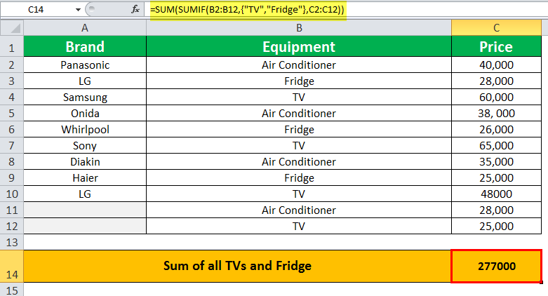
The following table shows the total amount calculated by adding the sum of the prices of two items - TV and fridge in the cell C14, using the SUMIF formula. The SUM of the prices of the fridges and TVs are 79,000 and 1,98,000,  respectively. Hence, the total SUM of the prices of two items is 2,77,000.

The SUMIF formula is applied to the range C2:C12 and is stated as follows:

“=SUM(SUMIF(B2:B12,{“TV”,“Fridge”},C2:C12))”

Where,

• B2: B12 refers to the range on which the criteria are to be applied.
• “TV,” “fridge” refers to the two individual conditions to be checked in range B2: B12. The curly braces {} of the criterion represent the collection of constants.
• C2: C12 refers to the range of values to be added.

In the formula, the SUMIF function is enclosed within the SUM function. The SUMIF formula executes two different conditions, “TV” and “fridge.” Finally, the SUM function sums the results of the SUMIF functions to return the output.

The guidelines of the argument of the SUMIF formula are stated as follows:

• The numeric criteria are not enclosed in double quotes.
• The text criteria for SUMIF, including the mathematical symbols, are enclosed within double quotes.
• The wildcard characters - question mark (?) and asterisk (*) used in the criteria match a single character and a series of characters, respectively.
• The tilde operator (~) followed by the wildcard characters refer to the actual characters. For example, the “~?” indicates criteria as a question mark literally.
• The SUMIF formula returns “#VALUE! error” when the criterion is a text string that is greater than 255 characters.