Table Of Contents

SUM Function in Excel

Last Updated :

Blog Author :

Edited by :

Reviewed by :

The Syntax of the SUM Excel Function

The syntax of the function is shown in the following image:

The function accepts the following arguments:

Number1: This is the first numeric value to be added.
Number2: This is the second numeric value to be added.

The “number1” argument is required while the subsequent numbers (“number 2”, “number 3”, etc.) are optional.

SUM Function in Excel Explained in Video

The Procedure to Enter the SUM Function in Excel

To enter the SUM function manually, type “=SUM” followed by the arguments.

The alternative steps to enter the SUM excel function are listed as follows:

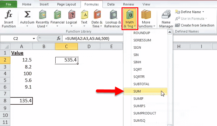
In the Formulas tab, click the “math & trig” option, as shown in the following image.

2. From the drop-down menu that opens, select the SUM option.

3. In the “function arguments” dialog box, enter the arguments of the SUM function. Click “Ok” to obtain the output.

The AutoSum Option in Excel

The AutoSum option is the fastest way to add numbers in a range of cells. It automatically enters the SUM formula in the selected cell.

Let us work on an example to understand the working of the AutoSum option. We want to sum the list of values in A2:A7, shown in the succeeding image.

The steps to use the AutoSum command are listed as follows:

Select the blank cell immediately following the cell to be summed up. Choose the cell A8.
In the Home tab, click “AutoSum”. Alternatively, press the shortcut keys “Alt+=” together and without the inverted commas.
The SUM formula appears in the selected cell. It shows the reference of the cells that have been summed up.
Press the “Enter” key. The output appears in cell A8, as shown in the following image.

How to Use the SUM Function in Excel?

Let us consider a few examples to understand the usage of the SUM function. The examples #1 to #5 show an image containing a list of numeric values.

Example #1

We want to sum the cells A2 and A3 shown in the succeeding image.

Apply the formula “=SUM(A2, A3).” It returns 20.7 in cell C2.

Example #2

We want to sum the cells A3, A5, and the number 45 shown in the succeeding image.

Apply the formula “=SUM (A3, A5, 45).” It returns 58.8 in cell C2.

Example #3

We want to sum the cells A2, A3, A4, A5, and A6 shown in the succeeding image.

Apply the formula “=SUM (A2:A6).” It returns 135.4 in cell C2.

Example #4

We want to sum the cells A2, A3, A5, and A6 shown in the succeeding image.

Apply the formula “=SUM (A2:A3, A5:A6).” It returns 35.4 in cell C2.

Example #5

We want to sum the cells A2, A3, A5, A6, and the number 500 shown in the succeeding image.

Apply the formula “=SUM (A2:A3, A5:A6, 500).” It returns 535.4 in cell C2.

The Usage of the SUM Excel Function

The rules governing the usage of the function are listed as follows:

The arguments supplied can be numbers, arrays, cell references, constants, ranges, and the results of other functions or formulas.
While providing a range of cells, only the first range (cell1:cell2) is required.
The output is numeric and represents the sum of values supplied.
The arguments supplied can go up to a total of 255.

Note: The SUM excel function returns the “#VALUE!” error if the criterion supplied is a text string longer than 255 characters.

The Limitations of the SUM Function in Excel

The drawbacks of the function are listed as follows:

The cell range supplied must match the dimensions of the source.
The cell containing the output must always be formatted as a number.

The Nesting of the SUM Excel Function

The built-in formulas of Excel can be expanded by nesting one or more functions inside another function. This permits multiple calculations to take place in a single cell of the worksheet.

The nested function acts as an argument of the main or the outermost function. Excel calculates the innermost function first and then moves outwards.

For example, the following formula shows the SUM function nested within the ROUND function:

For the given formula, the output is calculated as follows:

First, the sum of the values in cells A1 to A6 is computed.
Next, the resulting number is rounded to three decimal places.

With Microsoft Excel 2007, nested functions up to 64 levels are permitted. Prior to this version, one could nest functions only till 7 levels.

Frequently Asked Questions

1. Define the SUM function of Excel.

The SUM function helps add the numerical values. These values can be supplied to the function as numbers, cell references, or ranges. The SUM function is used when there is a need to find the total of specified cells.

The syntax of the SUM excel function is stated as follows:
“SUM(number1, ,…)”
The “number1” and “number2” are the first and second numeric values to be added. The “number1” argument is mandatory while the remaining values are optional.

In the SUM function, the range to be summed can be provided, which is easier than typing the cell references one by one. The AutoSum option provided in the Home or Formulas tab of Excel is the simplest way to sum two numbers.

Note: The numeric value provided as an argument can be either positive or negative.

2. How to sum the values of filtered data in Excel?

To add the values of filtered data, use the SUBTOTAL function. The syntax of the function is stated as follows:

“SUBTOTAL(function_num,ref1,,…)”

The “function_num” is a number ranging from 1 to 11 or 101 to 111. It indicates the function to be used for the SUBTOTAL. The functions used can be AVERAGE, MAX, MIN, COUNT, STDEV, SUM, and so on.

The “ref1” and “ref2” are the cells or ranges to be added.

The “function_num” and “ref1” arguments are mandatory. The “function_num” 109 is used for adding the visible cells of filtered data.

Let us consider an example.

• The sales revenue generated by A and B of team X are:
$1,240 and $3,562 given in cells C2 and C3 respectively

• The sales revenue generated by C and D of team Y are:
$2,351 and $4,109 given in cells C4 and C5 respectively

We filter only team X rows and apply the formula “SUBTOTAL(109,C2:C3).” It returns $4,802.

Note: Alternatively, the AutoSum property can be used to sum the filtered cells.

3. State the benefits of using the SUM function in Excel.

The benefits of using the SUM function are listed as follows:
• It helps obtain the totals of ranges irrespective of whether the cells are contiguous or non-contiguous.
• It ignores the empty cells and text values entered in a cell. In such cases, it returns an output representing the sum of the remaining numbers of the range.
• It automatically updates to include the addition of a row or a column.
• It automatically updates to exclude the deletion of a row or column.
• It eliminates the difficulty associated with typing manual entries.
• It makes the output more readable by allowing the cell to be formatted as a number.