SUBTOTAL Function in Excel

What is SUBTOTAL Function in Excel?

The SUBTOTAL excel function performs different arithmetic operations like average, product, sum, standard deviation, variance etc., on a defined range. Each operation has a unique function number assigned to it. This function number is supplied as an argument to the SUBTOTAL function.

For example, a worksheet consists of the following values in column A:

Cell A1 contains 22
Cell A2 contains 45
Cell A3 contains 37
Cell A4 contains 12

The formula “=SUBTOTAL(1,A1:A4)” returns 29. This output is the average of the given range (A1:A4). The number 1 in the formula tells Excel that the average of the listed numbers is to be calculated.

With the SUBTOTAL function, one can either include or exclude the values of the hidden rows. However, the filtered-out values (the values hidden by a filter) are excluded, by default.

The SUBTOTAL function works with vertical ranges (columns) of a dataset. It can perform 11 different arithmetic operations on a dataset. The SUBTOTAL function is categorized under the Math and Trigonometry functions of Excel.

The SUBTOTAL is a versatile function which is available in all versions of Excel. In the modern versions of Excel, the AGGREGATE functionAGGREGATE Function AGGREGATE Function in excel returns the aggregate of a given data table or data lists.read more is also available. This can perform more operations compared to the SUBTOTAL excel function.

Syntax of the SUBTOTAL in Excel

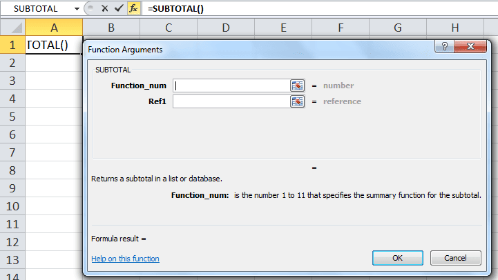
The syntax of the SUBTOTAL function of Excel is shown in the following image:

The SUBTOTAL function accepts the following arguments:

Function_num: This is the number that determines which arithmetic operation (function) will be performed by the SUBTOTAL function. The “function_num” argument can take any value from 1 to 11 or 101 to 111.
Ref1: This is the range of cells on which the arithmetic operation is to be performed. It can be supplied as a reference or as a named range.
Ref2: This is the second range of cells on which the arithmetic operation is to be performed. This also can be entered as a reference or as a named range.

The arguments “function_num” and “ref1” are mandatory, while “ref2” is optional. The SUBTOTAL function returns a numeric output.

Note: The “function_num” argument is always entered as a numeric value.

Operations Performed by the SUBTOTAL Function

The SUBTOTAL function performs an arithmetic operation depending on the value of the “function_num” argument. The operations (functions) performed by the SUBTOTAL function and the corresponding function numbers are listed as follows:

Function	function_num Includes hidden values	function_num Excludes hidden values
AVERAGE	1	101
COUNT	2	102
COUNTA	3	103
MAX	4	104
MIN	5	105
PRODUCT	6	106
STDEV	7	107
STDEVP	8	108
SUM	9	109
VAR	10	110
VARP	11	111

One must observe that for every operation (function), there are two values (like 1 and 101 for AVERAGE) of the “function_num” argument. The “function_num” argument can take either of these values depending on whether the hidden rows are included or excluded from the subtotals.

The values of the “function_num” argument have the following implications:

When the value of “function_num” is between 1-11, the SUBTOTAL includes the manually hidden rows in the calculations.
When the value of “function_num” is between 101-111, the SUBTOTAL excludes the manually hidden rows from the calculations.

The values of rows hidden by a filter are always excluded irrespective of the “function_num” argument.

Note: The user need not memorize the function numbers. This is because as soon as one begins to type the SUBTOTAL formula in a cell, Excel displays a list containing the different operations and the corresponding function numbers. To select the operation to be performed, double-click its name displayed in the list.

How to Open the SUBTOTAL Function in Excel?

You can download this SUBTOTAL Function Excel Template here – SUBTOTAL Function Excel Template

To open the SUBTOTAL excel function, enter “=SUBTOTAL” in the required cell, followed by the arguments of the function. Alternatively, the SUBTOTAL function can be opened from the Formulas tab of Excel. The steps for the same are listed as follows:

Select the cell in which the SUBTOTAL formula is to be entered.
From the Formulas tab, click the drop-down of “Math & Trig”. Select “SUBTOTAL”, as shown in the following image.
The “function arguments” dialog box opens, as shown in the following image. Enter the values for the arguments “function_num” and “ref1”. Once the cursor is placed inside the “ref1” box, the “ref2” box appears below it.

Click “Ok” to proceed. The output of the SUBTOTAL function will be displayed in the cell selected in step 1.

How to use the SUBTOTAL Function in Excel?

Let us consider some examples to understand the working of the SUBTOTAL function of Excel.

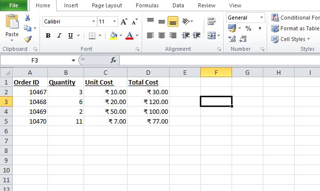
The succeeding image shows the IDs of four orders (in column A) received by an organization. Prior to completing these orders, the organization has compiled a dataset which contains the following information:

The quantities of goods to be supplied are listed in column B.
The unit costs of each good are given in column C.
The total costs of each order are shown in column D.

There are no hidden rows and filters in the given dataset. Perform the following tasks:

Apply all the 11 operations of the SUBTOTAL excel function to the range D2:D5. Cover one operation in one example. So, there must be 11 examples subsequent to the succeeding image.
At the end of example #11, the formulas and the results of all the examples must be consolidated at one place.

Let us begin with the different operations of the SUBTOTAL excel function covered in the following examples.

Note: Please ignore the small boxes containing question marks (in columns C and D) in the images of all the eleven examples.

Example #1

Let us apply the AVERAGE functionAVERAGE Function The AVERAGE function in Excel gives the arithmetic mean of the supplied set of numeric values. This formula is categorized as a Statistical Function. The average formula is =AVERAGE(read more with the SUBTOTAL formula. This helps calculate the average of the defined range. The steps for the same are listed as follows:

Step 1: Enter the following formula in cell F2.

“=SUBTOTAL(1,D2:D5)”

Note: To select the function number 1, double-click “1-AVERAGE” appearing in the list of the available arithmetic operations. Alternatively, one can type “1” (without the double quotation marks) manually.

Step 2: Press the “Enter” key. The output is 81.75, which appears in cell F2. The same is shown in the following image.

Explanation: The first argument of the given SUBTOTAL excel formula (entered in step 1) is 1, which implies that the average needs to be calculated. The second argument is the range D2:D5. So, the average is computed for the range D2:D5. Hence, the output of the formula is 81.75.

Since there are no hidden rows, we have used 1 as the function number. Had there been a hidden row, we would have applied the formula “=SUBTOTAL(101,D2:D5).” This formula would have excluded the hidden row and performed the given operation (average) on the visible rows of the range D2:D5.

For instance, if rows 3 and 5 had been hidden, the formula “=SUBTOTAL(101,D2:D5)” would have returned 65. This is the average of the numbers 30 and 100.

Example #2

Let us apply the COUNT functionCOUNT Function The COUNT function in excel counts the number of cells containing numerical values within the given range. It is a statistical function and returns an integer value. The syntax of the COUNT formula is “=COUNT(value 1, [value 2],…)” read more with the SUBTOTAL excel formula. This helps count the numeric values of the defined range. The steps are listed as follows:

Step 1: Enter the following formula in cell F2.

“=SUBTOTAL(2,D2:D5)”

Note: Double-click “2-COUNT” from the list of operations. In this way, the function number 2 appears in the SUBTOTAL formula.

Step 2: Press the “Enter” key. The output 4 appears in cell F2, as shown in the following image.

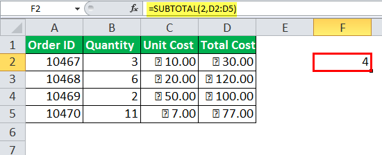
Explanation: The “function_num” is 2 and “ref1” is D2:D5. So, the COUNT function is applied to the range D2:D5. The COUNT function counts the number of cells containing numeric values in the range D2:D5.

There are four numeric cells in the range D2:D5. These cells are D2, D3, D4, and D5. Hence, the output of the SUBTOTAL function is 4.

Note: The COUNT function counts those cells of a range which contain numbers (positive and negative both), dates, times, decimal numbers, percentages, and so on. It does not count the empty cells, error values, logical values (Boolean values true and false), and text strings.

Example #3

Let us apply the COUNTA functionCOUNTA Function The COUNTA function is an inbuilt statistical excel function that counts the number of non-blank cells (not empty) in a cell range or the cell reference. For example, cells A1 and A3 contain values but, cell A2 is empty. The formula “=COUNTA(A1,A2,A3)” returns 2. read more with the SUBTOTAL excel formula. This helps count the non-blank cells of the defined range. The steps for the same are listed as follows:

Step 1: Enter the following formula in cell F2.

“=SUBTOTAL(3,D2:D5)”

Note: To enter 3 as the “function_num” in the SUBTOTAL formula, double-click “3-COUNTA” from the list displayed in Excel.

Step 2: Press the “Enter” key. The output is 4 in cell F2, as shown in the following image.

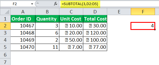
Explanation: The “function_num” argument is 3 and the “ref1” argument is D2:D5. The given SUBTOTAL formula (entered in step 1) counts the non-empty cells in the range D2:D5.

The non-empty cells in the given range (D2:D5) are D2, D3, D4, and D5. Hence, the output of the SUBTOTAL formula is 4.

Note: The COUNTA function counts the cells containing text strings, numbers, logical (Boolean) values, date/time values, error values, and so on. Only the absolutely empty cells are excluded from the count.

Example #4

Let us apply the MAX functionMAX Function The MAX Formula in Excel is used to calculate the maximum value from a set of data/array. It counts numbers but ignores empty cells, text, the logical values TRUE and FALSE, and text values.read more with the SUBTOTAL excel formula. This helps find the largest value of the defined range. The steps for the same are listed as follows:

Step 1: Enter the following formula in cell F2.

“=SUBTOTAL(4,D2:D5)”

Note: To select the “function_num” 4, double-click “4-MAX” from the list displayed in Excel. Alternatively, one can type “4” (without the double quotation marks) manually.

Step 2: Press the “Enter” key. The output in cell F2 is 120. It is shown in the following image.

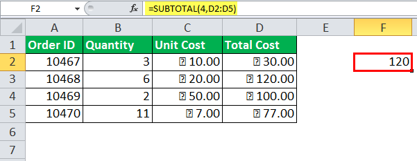
Explanation: The MAX function returns the largest numeric value from a series of numbers. With the given SUBTOTAL formula (entered in step 1), the largest value of the range D2:D5 is 120. Hence, the output is 120.

Had we hidden the rows 3 and 4, the formula “=SUBTOTAL(104,D2:D5)” would have returned 77. This is because 77 is the larger of the two visible values (30 and 77). So, the function number 104 excludes the values of the hidden rows while finding the maximum number of a range.

Note: The MAX function considers the numerical values of a dataset. If a range consists of text strings, logical values (true and false) or empty strings, they are ignored by the MAX function.

Example #5

Let us apply the MIN function with the SUBTOTAL excel formula. This helps find the smallest value of the defined range. The steps are listed as follows:

Step 1: Enter the following formula in cell F2.

“=SUBTOTAL(5,D2:D5)”

Note: Double-click “5-MIN” (in the list of functions) to enter 5 as the “function_num” argument.

Step 2: Press the “Enter” key. The output in cell F2 is 30, as shown in the following image.

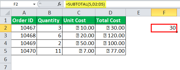
Explanation: The MIN function returns the smallest value from a list of numbers. Here, the smallest number of the range D2:D5 is 30.

Hence, the output of the SUBTOTAL formula (entered in step 1) is 30.

Note: Like the MAX function, the MIN also works with numerical values of a range. The MIN function ignores the text strings, empty strings, and logical values.

Example #6

Let us apply the PRODUCT functionPRODUCT Function Product excel function is an inbuilt mathematical function which is used to calculate the product or multiplication of the given numbers. If you provide this formula arguments as 2 and 3 as =PRODUCT(2,3) then the result displayed is 6.read more with the SUBTOTAL excel formula. This helps perform the multiplication of the defined range of numbers. The steps for the same are listed as follows:

Step 1: Enter the following formula in cell F2.

“=SUBTOTAL(6,D2:D5)”

Note: To enter 6 as the “function_num” argument, double-click “6-PRODUCT” from the list of functions.

Step 2: Press the “Enter” key. The output is 27720000. Since this number is quite big, we have retained its scientific notation in cell F2. For this, perform the following tasks:

Select cell F2 and right-click it.
Select “format cells” from the context menu.
Under “category,” select “scientific.” In “decimal places,” enter “1.”
Click “Ok.”

The scientific notation 2.8E+07 appears in cell F2, as shown in the following image. The SUBTOTAL formula can also be seen in the formula bar. The output 27720000 can be viewed in the image at the end of example #11, which shows the consolidated results.

Note 1: The scientific notation displays a number in the exponential format. In Excel, scientific notations are often used to shorten large numeric values. By using a scientific notation, the appearance of a cell value changes. However, the value itself does not change.

Note 2: The preview of the formatted number can be seen under “sample” in the “format cells” dialog box.

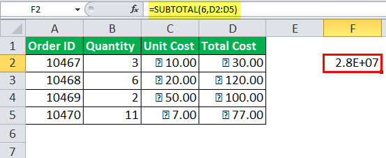
Explanation: The SUBTOTAL formula (entered in step 1) performs the multiplication operation on the range D2:D5. This works as follows:

30*120*100*77=27720000

Hence, the output (27720000) is the product of the numbers in cells D2, D3, D4, and D5.

Had we hidden the rows 3 and 4, the formula “=SUBTOTAL(106,D2:D5)” would have returned 2310. This is the product of the visible cells D2 and D5.

Example #7

Let us apply the STDEV or STDEV.S functionSTDEV.S Function The standard deviation shows the variability of the data values from the mean (average). In Excel, the STDEV and STDEV.S calculate sample standard deviation while STDEVP and STDEV.P calculate population standard deviation. STDEV is available in Excel 2007 and the previous versions. However, STDEV.P and STDEV.S are only available in Excel 2010 and subsequent versions. read more with the SUBTOTAL excel formula. This helps calculate the standard deviation of a population based on a data sample. The steps for the same are listed as follows:

Step 1: Enter the following formula in cell F2.

“=SUBTOTAL(7,D2:D5)”

Note: Double-click “7-STDEV” or “7-STDEV.S” to select the function number 7.

Step 2: Press the “Enter” key. The output is 38.7158, as shown in the following image.

Note: Population refers to the entire dataset, while a sample is a subset of this dataset. In other words, a sample contains one or more elements of the population.

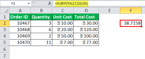
Explanation: The STDEV and STDEV.S calculate the standard deviation by assuming the range D2:D5 as a sample of the population. Hence, the sample standard deviation is 38.7158. This is the output of the SUBTOTAL formula entered in step 1.

While calculating the sample standard deviation, “n-1” is taken as the denominator, where “n” is the number of values in a dataset.

The high standard deviation (38.7158) implies that the values of the given range (D2:D5) fluctuate from the mean (average) to a great extent.

Note 1: The standard deviation indicates the dispersion (deviation) of the data values from the mean (average). In other words, with standard deviation, one can say whether the data values are close or spread out from the mean.

Note 2: Both STDEV and STDEV.S are sample standard deviations that help make relevant conclusions for the population. The STDEV.S is an improved version of the STDEV function. STDEV.S is available in Excel 2010 and the subsequent versions.

Note 3: Both STDEV and STDEV.S ignore the text strings and the logical values of the data sample.

Example #8

Let us apply the STDEVP or STDEV.P function with the SUBTOTAL excel formula. This helps calculate the standard deviation of the entire population. The steps are listed as follows:

Step 1: In cell F2, enter the following formula.

“=SUBTOTAL(8,D2:D5)”

Note: Double-click “8-STDEVP” or “8-STDEV.P” to enter function number 8. Alternatively, one can type “8” (without the double quotation marks) manually.

Step 2: Press the “Enter” key. The output in cell F2 is 33.5289. The same is shown in the following image.

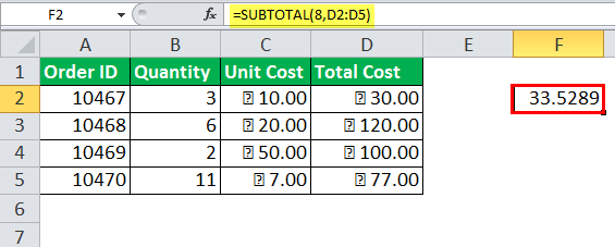
Explanation: The STDEVP and STDEV.P functions assume that the data supplied as an argument (range D2:D5) represents the entire population. Hence, the SUBTOTAL formula (entered in step 1) returns the population standard deviation, which is 33.5289.

While calculating the population standard deviation, “n” is taken as the denominator, where “n” is the number of values in a dataset.

The high standard deviation (33.5289) indicates high variability of the supplied values (range D2:D5) from the mean (average).

Note: Both the STDEVP and STDEV.P functions ignore the text strings and logical values of the population dataset. The STDEV.P is an improved version of STDEVP. The STDEV.P function is available in Excel 2010 and the newer versions.

Example #9

Let us apply the SUM functionSUM Function The SUM function in excel adds the numerical values in a range of cells. Being categorized under the Math and Trigonometry function, it is entered by typing “=SUM” followed by the values to be summed. The values supplied to the function can be numbers, cell references or ranges.read more with the SUBTOTAL excel formula. This helps to sum up the numeric values of the defined range. The steps are listed as follows:

Step 1: In cell F2, enter the following formula.

“=SUBTOTAL(9,D2:D5)”

Note: To enter function number 9, double-click “9-SUM” displayed in the Excel list of functions. Alternatively, type the number “9” (without the double quotation marks) manually.

Step 2: Press the “Enter” key. The output in cell F2 is 327. It is shown in the following image.

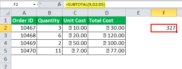
Explanation: The SUM function adds the values of the range D2:D5. It works as follows:

30+120+100+77=327

Hence, the output of the SUBTOTAL formula (entered in step 1) is 327.

Had we hidden the rows 3 and 4, the formula “=SUBTOTAL(109,D2:D5)” would have returned 107. This addition considers the values of the visible cells (D2 and D5) only.

Note: The SUM function ignores the empty cells and the text strings of the dataset.

Example #10

Let us apply the VAR or VAR.S function with the SUBTOTAL excel function. This calculates the variance of a population based on a data sample. The steps for the same are listed as follows:

Step 1: Enter the following formula in cell F2.

“=SUBTOTAL(10,D2:D5)”

Note: To enter 10 in the SUBTOTAL formula, double-click “10-VAR” or “10-VAR.S” from the list of functions.

Step 2: Press the “Enter” key. The output is 1498.92, as shown in the following image.

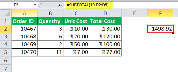
Explanation: The VAR and VAR.S functions assume that the values supplied (range D2:D5) as an argument are a sample of the population. Hence, the sample variance returned by the SUBTOTAL formula (entered in step 1) is 1498.92.

Since the output (1498.92) is large, it indicates high variance or high volatility (risk). When the variance is high, the following is inferred:

The sample values (range D2:D5) supplied are far from the mean (average).
The sample values are more spread out from each other.

Note 1: The sample variance is the square of the sample standard deviation. When the variance is zero (output of the SUBTOTAL formula is 0), there is no variability in the values of the dataset. This implies that all the values of the dataset are identical.

Note 2: The VAR and VAR.S ignore the text strings and the logical values of the data sample. The VAR.S is an improved version of the VAR function. The VAR.S is available in Excel 2010 and all the subsequent versions.

Example #11

Let us apply the VARP or VAR.P function with the SUBTOTAL excel formula. This helps calculate the variance of the entire population. The steps for the same are listed as follows:

Step 1: In cell F2, enter the following formula.

“=SUBTOTAL(11,D2:D5)”

Note: Double-click “11-VARP” or “11-VAR.P” to enter 11 in the SUBTOTAL formula. Alternatively, one can type “11” (without the double quotation marks) manually.

Step 2: Press the “Enter” key. The output appears in cell F2. It is 1124.19, as shown in the following image.

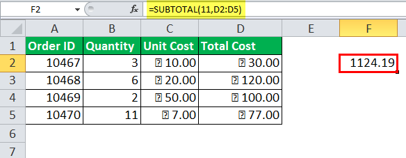
Explanation: The VARP and the VAR.P functions assume that the supplied values (range D2:D5) represent the entire population. Hence, the output of the SUBTOTAL formula (entered in step 1) is the population variance. This figure is 1124.19.

The output (1124.19) is large, which implies that the values of the entire population (range D2:D5) are scattered (spread out). A high variance is associated with high volatility (risk).

Note: The population variance is the square of the population standard deviation. The VAR.P is an improved version of VARP. The VAR.P is available in Excel 2010 and the subsequent versions. The VARP and VAR.P both ignore the text strings and the logical values of the population dataset.

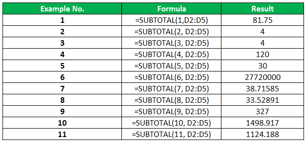
Let us consolidate the results of the preceding examples (example #1 to #11) in the succeeding image.

The formulas and the outputs are shown in the columns “formula” and “result” respectively. The example numbers (1-11) are shown in the first column titled “example no.”

Properties

The major features of the SUBTOTAL excel function are listed as follows:

Property 1: The SUBTOTAL function, with function number between 101-111, does not work with horizontal ranges. For instance, a worksheet contains the following data:

Cell A1 contains 2

Cell B1 contains 3

Cell C1 contains 4

Cell D1 contains 5

The formula “=SUBTOTAL(106,A1:D1)” returns 120. If column C is hidden, the formula “=SUBTOTAL(106,A1:D1)” returns 120 again. This implies that while performing an operation on a horizontal range, hiding a column does not impact the SUBTOTAL excel function.

However, hiding a row, while performing an operation on a vertical range, does impact the SUBTOTAL formula. This is true when the function number is between 101-111. In this case, the SUBTOTAL formula calculates an output by considering only the visible rows.

Hence, when the function number is between 101-111, the SUBTOTAL function works as follows:

It includes the values of the hidden columns while working on a horizontal range.
It excludes the values of the hidden rows while working on a vertical range.

Property 2: The SUBTOTAL excel function ignores the nested SUBTOTAL formulas while performing an arithmetic operation. This is done to prevent errors that may occur as a result of double counting.

Note 1: A nested function is one which is placed inside another function. The inner (nested) function is calculated first. The outcome of the inner function becomes an argument for the outer function.

Note 2: Double counting is an error whereby the same number is counted twice.

Errors Returned by the SUBTOTAL Function

The SUBTOTAL excel function returns the following errors:

“#VALUE!” error: This error occurs due to either of the following reasons:
- If the function_num argument is not a permissible value (accepted values are integers between 1-11 or 101-111)
- If the range address supplied is a 3-D reference
“#DIV/0!” error: This error occurs due to either of the following reasons:
- If a calculation involves division by zero
- If a function (arithmetic operation) works with only numbers, but the defined range does not contain any numeric value
“#NAME?” error: This error occurs if the name of the SUBTOTAL function is spelt incorrectly.

Note: In a 3-D reference, the same range (or a cell) is referred on various worksheets. For instance, the reference Sheet1:Sheet3!A1:A5 is a 3-D reference of the range A1:A5. This reference involves the worksheets, “Sheet1,” “Sheet2, and “Sheet3.”

Frequently Asked Questions

1. Define the SUBTOTAL function of Excel.

The SUBTOTAL function performs a specified arithmetic operation (like average, minimum, maximum, count, product etc.) on a pre-defined range of cells. A total of 11 different operations can be performed by the SUBTOTAL function. Further, this function works with vertical ranges of a dataset.

The syntax of the SUBTOTAL function is stated as follows:

“SUBTOTAL(function_num,ref1,[ref2],…)”

The “function_num” is used to specify the operation (function) that will be performed by the SUBTOTAL function. The “ref1” and “ref2” are the first and the second range of cells respectively on which the operation is to be performed.

The “function_num” and “ref1” are mandatory arguments, while “ref2” is an optional argument. The function number 1-11 includes the rows hidden manually, while 101-111 excludes the values of hidden rows. The values of rows hidden by a filter are always excluded.

As a user begins to enter the SUBTOTAL formula in a cell, Excel displays a list of the available function numbers. One can double-click the required function number to select it.

2. Why is the SUBTOTAL function used in Excel?

The SUBTOTAL function is used for the following reasons:

a. It produces dynamic results in the case of filtered data. Once a filter is applied, the SUBTOTAL formula (with function number 101-111) automatically recalculates to include only the values visible after filtering. So, the output of the SUBTOTAL formula corresponds to the filters applied.
b. It ignores the values of the manually hidden rows. When one or more rows are hidden, the SUBTOTAL formula excludes such rows from the calculations. In this way, the arithmetic operations can be performed only on the relevant data.
c. It ignores the nested SUBTOTAL formulas. If a user has applied multiple SUBTOTAL formulas to the same range, only the outer subtotals are calculated. The inner (nested) subtotals are excluded from the calculations. In this way, several operations can be performed on the same range, without worrying about double counting.
d. It helps perform various arithmetic operations by using a single function. Had different functions been used for the different operations, the arguments of each function had to be remembered. So, the usage of the SUBTOTAL function eases working with Excel.

3. Where is the SUBTOTAL function in Excel?

In Excel, the SUBTOTAL function can be accessed in the following ways:

Method 1

a. Begin by typing “=SUBTOTAL” directly in a cell.
b. Type the function number and select the range on which the operation is to be performed.
c. Press the “Enter” key.

Method 2

a. Select a cell in which the subtotals are to be calculated.
b. Click the drop-down arrow of Math and Trigonometry from the Formulas tab. Select “subtotal”.
c. The “function arguments” dialog box appears. In this, enter the desired function number and the range on which the operation is to be performed.
d. Click “Ok” to apply the SUBTOTAL function.

Method 3

a. Select the dataset on which the SUBTOTAL function is to be applied.
b. From the Data tab, click “subtotal”. The “subtotal” dialog box appears.
c. In the box below “at each change in”, select the column whose entries are to be consolidated or grouped. The name of the operation will appear in this column after each group of rows.
d. In the box below “use function”, select the operation to be performed.
e. In the box below “add subtotal to”, select the column to which the SUBTOTAL formula should be applied. This column should contain the values that are to be subtotaled.
f. Select or deselect the following checkboxes:
• “Summary below data” – Select this checkbox if a summary row is required immediately below the dataset. If the summary row should be right below the column headers, deselect this checkbox.
• “Replace current subtotals” – Deselect this checkbox to prevent overwriting the already existing subtotals. In case there are no existing subtotal formulas, one may or may not select this checkbox.
• “Page break between groups” – Select this checkbox if the page breaks at the end of each subtotal are required.
g. Click “Ok” to apply the SUBTOTAL function.

The “plus” (+) and “minus” (-) boxes are created to the left side of the worksheet. These boxes can be used to expand or collapse the rows of the dataset.

Note: For method 3 to work correctly, ensure that every column has a label or header in the first row of the dataset. It is not advised to have blank rows or columns in the range on which the subtotals are to be applied.

19th/20th September 2020	Saturday - Sunday	9 am IST to 5 pm IST
26th/27th September 2020	Saturday - Sunday	9 am IST to 5 pm IST

SUBTOTAL Function in Excel