Substring In Excel

The SUBSTRING function is a pre-built integrated function in Excel that is categorized under the TEXT function. Substring means extracting a string from a combination of strings. Unfortunately, there is no built-in function to extract a substring in Excel, but we can use other functions such as the MID or LEFT and RIGHT functions

For example, consider the below table showing text string in cell A1.

Now, let us extract the text 38 from right using RIGHT function.

The formula is =RIGHT(A1,2). Press Enter key.

We can see the result as shown in the below image.

1. SUBSTRING function in Excel is a ready-made built-in function that extracts a string from a combination of strings. It is classified as a TEXT function. Excel does not have a built-in function to extract substrings, but you can use other functions such as MID, LEFT, and RIGHT.
2. The three types of substring functions are LEFT, RIGHT, and MID-SUBstring functions.
3. The RIGHT function is used to extract domain names from email addresses, while SUBSTRING functions remove first, middle, and last names from full names, remove trailing slashes in web URLs, and extract country or state code from phone numbers.

1. LEFT Substring Function
2. RIGHT Substring Function
3. MID Substring Function

Let us discuss each one in detail.

#1 - Extract Text From The Left Of A String

It extracts a specific number of characters from the left side or first character of a supplied text string.

The syntax or formula for the LEFT function in Microsoft Excel is:

The LEFT function syntax or formula has the below-mentioned arguments:

• text: (Compulsory or required parameter) The text string contains the characters you want to extract.
• num_chars: (Optional parameter) It is the number of characters from the left side of the text string which you want to extract.
• For Example, =LEFT(“application,” 3) returns the 3 number of characters from the left side, i.e., “app.”

Points to Remember about LEFT Function

• In the LEFT and RIGHT function, num_chars must be equal to OR greater than zero. Otherwise, it returns a #VALUE! Error.
• If the num_chars argument in the LEFT or RIGHT function is greater than the length of text, LEFT returns all of the text. For example, =LEFT (“FUNCTION,” 25) returns “FUNCTION.”
• If the num_chars argument in the left or right function is omitted, it will consider or assume 1 by default. For example,  =LEFT(“Swift”) returns “S.”

#2 - Get Text From The Right Of A String

It extracts a specific number of characters from the RIGHT side of a supplied text string.

The syntax or formula for the RIGHT function in Microsoft Excel is:

The RIGHT function syntax or formula has the below-mentioned arguments:

• Text: (Compulsory or required parameter) It is the Text string that contains the characters where you want to extract.
• num_chars: (Optional parameter) The number of characters from the RIGHT side of the text string you want to remove.
• For Example, =RIGHT(“application,” 6) returns the 6 number of characters from the right side, i.e., “cation.”

#3 - Extract Text From The Middle Of A String

It extracts a specific number of characters from the middle part of a supplied text string.

The syntax or formula for the MID function in Excel is:

All the arguments are compulsory and require parameters.

The MID function syntax or formula has the below-mentioned arguments:

• Text: It is the text string that contains the characters that you want to extract.
• start_num: It specifies the position of the first character or starting position of the substring from where you want to begin.
• num_chars: The number of characters from the middle part of the text string you want to extract. (begins with start_num).
• For Example, =MID(“majori,” 2,5) returns the substring from the second character and 5 letters or alphabet from the second character, “ajori.”

Points to Remember

• If start_num is greater than the length of the text, then the MID function returns an empty value.
• If start_num is less than 1, then the MID function returns #VALUE! Error.
• If num_chars is a negative value, then the MID function returns #VALUE! Error.

Let us look at how the SUBSTRING functions work in Excel.

Example #1

In the below-mentioned example, cell “B3” contains the employee ID with the name. Here, we need to extract only employee ID with the help of the LEFT FUNCTION.

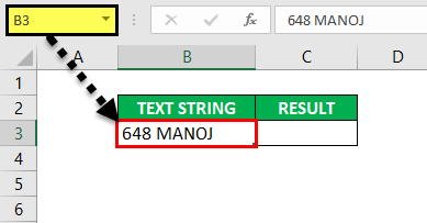
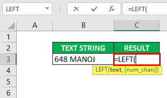
Let us apply the “LEFT” function in cell “C3”. Type =LEFT( in the cell “C3” where arguments for the LEFT function will appear. i.e. =LEFT (text, ) it needs to be entered.

Text: The text string contains the characters where you want to extract substring Excel, i.e., “B3” or “648 MANOJ.”

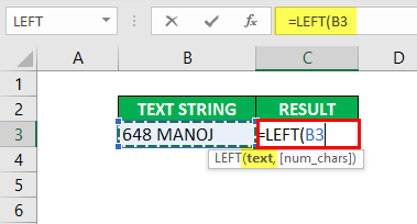
num_chars: The number of characters from the left side of the text string you want to extract. Here, the employee ID contains 3 numbers, so we only want to remove the first three numbers.

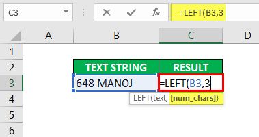
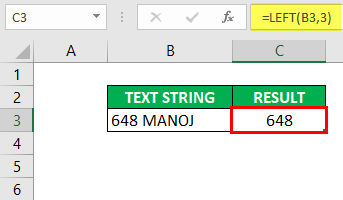
Click the "ENTER" key after entering all the LEFT function arguments: =LEFT(B3,3).

It extracts the first 3 characters from the text, 648.

Example #2

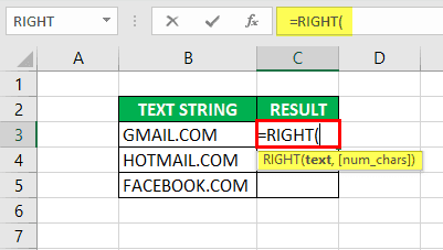
The below-mentioned example contains domain or website names. Here, we need to extract the last three characters with the help of the RIGHT function.

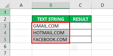
Let us apply the RIGHT function in cell “C3”. Type =RIGHT( in the cell “C3,” where arguments for the RIGHT function will appear: =RIGHT (text, ) it needs to be entered.

Text: The text string contains the characters where you want to extract substring Excel, i.e., “B3” or “GMAIL.COM.”

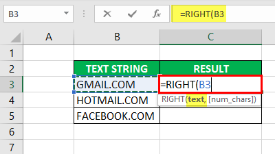
num_chars: It is the number of characters from the right side of the text string you want to extract. Here, all the website name ends with “COM,” so we want only the last three characters.

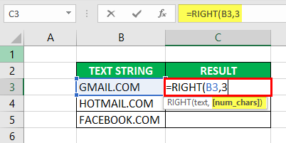
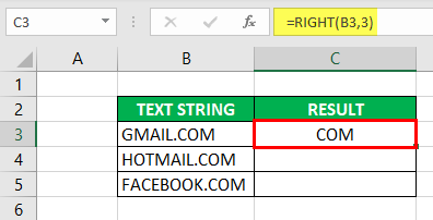
Click the "Enter" key after entering the RIGHT function: =RIGHT(B3,3).

Similarly, it is applied to other cells. You can also use the "drag & drop" option to get the desired output.

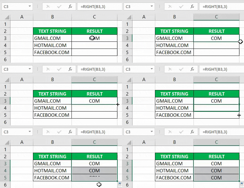
It extracts the last 3 characters from the text, COM.

Example #3

In the below-mentioned example, cell “B3” contains a PHONE NUMBER with an area code. Here, we need to extract only area code with the help of MID FUNCTION.

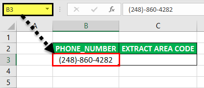
Let us apply the MID function in cell “C3”. Type =MID( in the cell “C3” where arguments for the MID function will appear. i.e. =MID(text,start_num,num_chars) it needs to be entered.

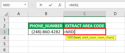
Text: It is the text string that contains the characters where you want to extract substring excel, i.e., “G14” or “(248)-860-4282.”

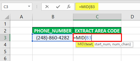
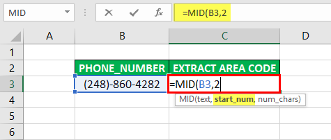
start_num: It specifies the position of the first character or starting position of the substring from where you want to begin, i.e., in the phone number, numbers in the bracket are the area code. We want only those numbers inside the bracket, i.e., 248. Here, the number inside the bracket begins from the 2nd position.

num_chars: The number of characters from the middle part of the text string you want to extract. (it begins with start_num). We want only those 3 numbers where area code is present inside the bracket, i.e., 3 characters.

Click the "Enter" key after entering all the MID function arguments: =MID(B3,2,3).

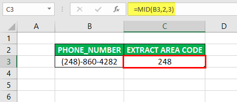
It extracts the 3 characters or numbers present inside the bracket, 248.

In Excel, there is no such thing as Substring function, by default. However, we can find substring in Excel using functions such as LEFT, RIGHT, MID functions.

Similarly, to extract specific functions, we can use FIND and SEARCH functions.

The SUBSTRING Excel function has wide applications:

• It is used to obtain the domain name from an email address with the help of the RIGHT function.
• It is used to get the first, middle, and last name from the full name with SUBSTRING functions.
• It is used to remove the trailing slash in web urls.
• It is used to extract country or state code from the phone number.

This article has been a guide to SUBSTRING in Excel. Here, we discuss how to use SUBSTRING functions in Excel: LEFT, MID, and RIGHT along with Excel examples and downloadable Excel templates. You may also look at these useful Excel tools: -

• String Functions in Excel VBA
• ISNA Function
• STRING to Date in VBA
• VBA Substring