Subscript in Excel

Last Updated :

Blog Author :

Edited by :

Reviewed by :

Table Of Contents

How To Do Subscripts in Excel?

Subscript in Excel is a formatting option in our data where we can make text and numbers look smaller. To do this, we need to right-click on the cell and, from the "Format Cells" tab in the "Font" section, check the "Subscript" option. Subscripts appear below the rest of the text. Although there is no shortcut for inserting a subscript in Excel in its technical sense, we can achieve this with a few key combinations.

How To Do Subscripts in Excel?

Shortcut for Subscript in Excel

The Excel subscript shortcut "Ctrl + 1, Alt + B, and Enter" format expressions such as "CH4" in your Excel spreadsheet. It requires using subscripts to convert it into the proper format, "CH4".

How to use This Excel Subscript Shortcut? (3 Easy Steps)

Please be careful not to click the keys at once. Each key combination should be pressed and released in turn.

Below are the steps for using the Excel subscript shortcut:

First, choose a character or more that you want to format.
Then, to open the "Format Cells" dialog, press "Ctrl + 1."
Then, press "Alt+B" to select the "Subscript" option, press the "Enter" key to apply the formatting and close the dialog box.

Examples

Let us understand the working of subscripts with the below examples. The subscript is very simple, can be used in an Excel worksheet on any character/number, and can be used in VBA.

Example #1

You can apply the subscript by using the below two methods in any cell of an Excel sheet.

Method 1:

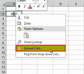
Step 1: Double click on cell A2 and select the value "2."

Step 2: Then right-click, and select "Format Cells."

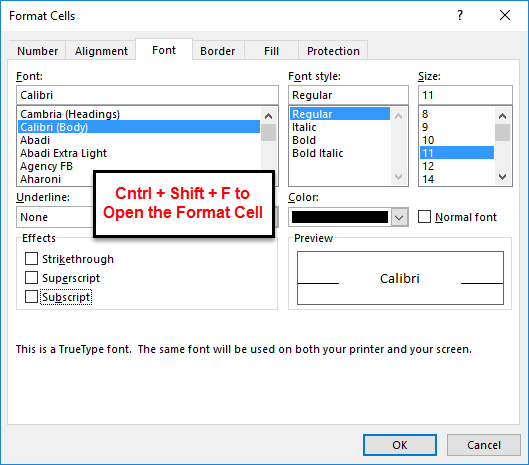
Step 3: The "Format Cells" dialog box appears.

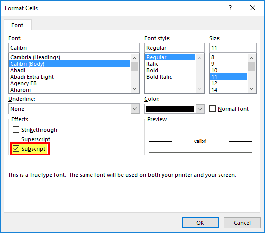
Step 4: On the "Font" tab, under the "Effect" checkmark on “Subscript,” then click on "OK."

Step 5: Then, it will convert the H2O to H₂O

Method 2:

The second method is to select a cell and the work directly in the formula bar.

Step 1: As before, carefully select the text you want to format. Then, use "Format Cells" to apply subscripts as you like.

Step 2: You can reverse or remove the subscript formatting by selecting the cell, accessing "Format Cells," and clearing the appropriate checkbox.

Subscript in Excel Example 1-1 (method 2)

Example #2

In this example, we are applying the subscript to CH4.

This time we are using the second method. Select the "4" from the formula bar, right-click, and click on "Format Cells."

("Format Cells" dialog box appears) then checkmark on "Subscript." That's it.

Now the output will be CH_4.

Example #3

A subscript is also used to distinguish between different types of subatomic particles. Thus, electron, muon, and tau neutrinos are denoted νe, νμ, and ντ.

Let us convert ve, Vu, and vτ to νe, νμ, and ντ in Excel.

Open the "Format Cells" dialog by pressing "Ctrl + 1" or right-click the selection and choose "Format Cells."

In the "Format Cells" dialog box, go to the "Font" tab and select "Subscript" under "Effects."

Click "OK" to save the change and close the dialog.

Example #4

You can also convert the whole-cell text to subscript.

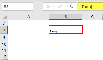
Select the cell, press "Ctrl+1," and then select the "Subscript" under "Effects."

How to use a keyboard shortcut to convert the selected cell text to subscript at once?

Press "Ctrl + Shift + F" to open the "Format Cells."

Press "ALT + B," and automatically select the "Subscript" option under the "Effects" and press the "Enter" key. Then, the text for the selected cell will automatically be converted to the subscript.

The result will be:

Subscript using VBA Code

Suppose we have the text in sheet1 and the D2 cell, then apply the subscript using the VBA code below.

Step 1: Go to the Developer tab and select the "Visual Basic" option.

Step 2: Create a function with any name and apply the below code, then run this macro to convert the D2 cell value to subscript.

Sub Subscripts ()

Range("D2").Characters(2, 1).Font.Subscript = True

MsgBox “D2 cell value in now in subscripts.”

End Sub

The result will be:

Things to Remember

Adding subscripts to Excel is usually a simple matter of a font setting, but you may run into limitations when adding subscripts to cells containing numbers or Excel formulas. We can work around this limitation by converting the data to text before adding the subscripts.