Strikethrough Text In Excel

Strikethrough text in Excel is a line that goes through or between the texts in an Excel cell, which means we strike the text.

We can use the Excel Strikethrough from the “Format” option of any cell by right-clicking on it and enabling the option or checkbox for Strikethrough, which will draw a line on the text, or use the keyboard shortcut, “CTRL+5”.

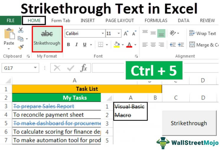
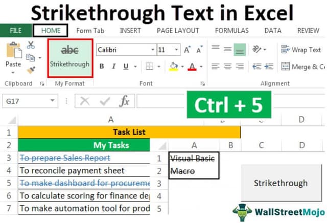
For example, in the following image, we have applied the Strikethrough Text feature for cells A3 and A5. Also, on the Visual Basic Macro text, on the inserted image.

We will consider 6 different methods to apply the Strikethrough Text In Excel, namely:

1. Strikethrough Text using Shortcut Key.
2. Using the Format Options.
3. By Adding the Strikethrough Button to Quick Access Toolbar.
4. Adding the Strikethrough Button to the Ribbon.
5. Using Conditional Formatting to Strikethrough automatically.
6. Adding a Button for Strikethrough Using VBA.

Now, let us discuss each of the methods with an example.

Method #1 - Strikethrough Text Using the Shortcut Key

We have a project, and the steps to be carried out are given in the below image.

As we will complete each step, we want to Strikethrough the steps that mark the completed status.

The steps to apply the Strikethrough using the shortcut keys are,

1. Select one or more cells using the “Shift” key with the “Up,” “Down,” “Left,” and “Right” arrow keys, and press the “Ctrl+5” keys.

   
   
   
   In our example, we do not have a requirement to highlight only some part of the value in the cell. Otherwise, we need to go into “Edit Mode” for the particular cell by double-clicking on the cell or using the “F2” key, selecting the text, and pressing the “Ctrl+5” keys.

2. Press the “F2” key to enter edit mode or double-click on the cell.

   
   

3. Press the “Ctrl+5” keys to Strikethrough the text.

   
   

4. Press the “Enter” key to get out of the edit mode.

   
   

Method #2 - Using the Format Options

Suppose we have the following data for steps. We want to Strikethrough the value as we complete each step.

The steps to apply the Strikethrough using the Format options are,

• Step 1 -  Select one or more cells on which we want to apply the Strikethrough, here, cell A3.

• Step 2 - Press the shortcut key “Ctrl + 1,” or right-click the selected cell(s), and choose “Format Cells” from the pop-up menu.

• Step 3 - In the “Format Cells” dialog box, we need to go to the “Font” tab, tick off the “Strikethrough” option under “Effects”, and then click “OK” to save the changes and close the dialog box.

Now, you can see the result as shown in the below image.

Method #3 - By Adding the Strikethrough Button to Quick Access Toolbar

Adding the “Strikethrough” button to the  Quick Access toolbar is a one-time setup, and we can use the button from QAT (Quick Access Toolbar) whenever required.

The steps to add the button to the QAT are:

• Step 1 - Right-click on the ribbon, and choose “Customize Quick Access Toolbar” from the pop-up menu.

• Step 2 - The “Excel Options” dialog box appears. Now, choose “Commands Not in the Ribbon” for “Choose commands from.”

• Step 3 - From the list, choose “Strikethrough”, and click the “Add” button to add the command button to the Quick Access Toolbar.

• Step 4 - We can use the up and down arrow buttons on the right side to change the position of the Strikethrough button. We have changed the position of the “Strikethrough” button to the fourth on the QAT. Click “OK.”

• Step 5 - We can find the “Strikethrough” command at fourth place on the QAT. As the command is at the fourth position, we can use Alt+4 as a shortcut excel key to apply the Strikethrough format to the selected text.

Method #4 - Adding the Strikethrough Button to the Ribbon

The Strikethrough command is not available on the MS Excel ribbon by default. We can find the same in the “Format Cells” dialog box. However, we can add the same command on the ribbon too. The steps to add the Strikethrough button are:

• Step 1 - Right-click anywhere on the ribbon, and choose “Customize the Ribbon…” from the pop-up menu.

• Step 2 - Choose “Commands Not in the Ribbon” for “Choose commands from” and select “Strikethrough” from the list.

• Step 3 - Before adding the “Strikethrough” command on the ribbon, first create the group using the “New Group” using the following steps,
  1. Select the tab under which you want to create the group. (In this case, the tab is the “Home” tab)
  2. Click on “New Group.”
  3. Rename the group using “Rename.”

• Step 4 - Add the “Strikethrough” command in the new group (My Format (Custom).”

• Step 5 - We can change the group’s position using the up and down arrow button on the right side of the dialog box, then click “OK.”

• We can see a new “My Format” group under the “Home” tab.

• We will format some of the text with Strikethrough for the following data.

To Strikethrough the values, the steps are:

• Select the cells we need to format, then choose the “Strikethrough” command from the “My Format” group under the “Home” tab.

Method #5 - Using Conditional Formatting to Strikethrough Automatically

We can Strikethrough the Text using conditional formatting in excel.

Suppose we have a task list that we need to accomplish. Then, we can update the status for the task as “Done”. We will format the task value with a Strikethrough, and the font color will automatically change to blue.

To do the same, the steps are:

• Step 1 - Select the cells to format.

• Step 2 - Go to the “Home” tab. From the “Styles” group, choose “Conditional Formatting.” Next, select “New Rule” from the drop-down list in excel.

• Step 3 - Choose “Use a formula to determine which cells to format.”

• Step 4 - For “Format values where this formula is true”. Specify =$B3=“Done”, and set the format as below.

• Step 5 - Click “OK” for both the dialog boxes, “Format Cells” and “New Formatting Rules.”

Now, whenever we update the status for a task as “Done”, the value is formatted.

Method #6 - Adding a Button for Strikethrough Using VBA

We can also create a command button for the same using VBA.

The steps to add a Strikethrough button using VBA are:

• Step 1 - Choose the “Command button” from the “Insert” command available in the “Controls” group under the Developer tab excel.

• Step 2 - Create the command button, and change the “Properties”, as shown in the images below.

• Step 3 - Click “View Code” from the “Controls” group after closing the properties dialog box. (Ensure the button is selected and “Design Mode” is activated.)

• Step 4 - Choose “Strikethrough” from the list.

• Step 5 - Save the file with .xlsm

Suppose we want to Strikethrough two cells (A1 and A2). We can do the same by selecting the cells and pressing the command button (make sure the “Design Mode” is deactivated).

Select the cells, and click the button.

• In a cell, we can apply the Strikethrough Text in Excel, even to just an alphabet or a character.

For example, My Name is John.

• It does not alter the cell’s value. Only the horizontal line appears. For example, “TEXT” and “TEXT” are equal.
• We can apply this feature by creating a “New Rule” using “Conditional Formatting”.