Table Of Contents
How to Sort by Numbers in Excel?

In this article, we will take you through Excel's method of sorting numbers. Believe us. Not many people do not know about this cool technique. So, why are you waiting to go one step more than your other counterparts?
We can find the "SORT" option in Excel under the "Data" tab. While sorting, we may need to sort on a column in one scenario. In some cases, we may be required to sort multiple columns simultaneously.
Sort by Number in Excel - Step by Step Guide
Here, we will learn how to sort by number in Excel.
Sort Numbers in Excel Example #1 - Single Level Sorting
A single-level sorting is nothing but sorting only one column at a time. For example, sorting by employee name is one-level sorting.
We have sales data based on the product. It includes product names and how many units are sold in a month. From largest to smallest, we want to sort based on the "Units Sold" column.

Below are the steps used for sorting numbers in Excel:
- First, select the data from A1 to B28.

- Go to the "Data" tab and "Sort." Use the shortcut key in Excel to open the "Sort" option. The shortcut key is "ALT + D + S."

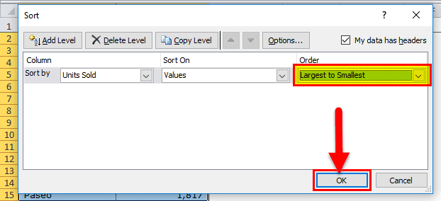
- Now, the mandatory thing: make sure the “My data has headers” checkbox has been ticked. If this box has been ticked, the selected data has headers. Otherwise, your will header will be treated as the data only.

- Click on the "Sort by" dropdown list and select the word "Units Sold."

- After this, undergo the "Order" section and select "Largest to Smallest." By default, Excel sets the order a "Smallest to Largest," but we can change it according to the requirement.

- Click on "OK" to sort the data from largest to smallest. The below image is the result of that.

Sort Numbers in Excel Example #2 - Multi-Level Sorting
The multi-level sorting includes many columns to sort at one. Sort by employee name and by department name. The employee name is one layer, and the department is another.
Let us take one more example to understand better. This example shows sales data across four regions at different time frames.

The first column includes "Dates," the second column consists of the "Region" name, and the third column contains "Revenue" numbers.
Now, we are required to sort region-wise. Also, we want to sort the revenue number from largest to smallest.
It is not a single-layer sort. It is a multi-level sorting. We need to include:
Step 1: Select the data first.

Step 2: Open the "Sort" box by pressing "ALT + D + S."

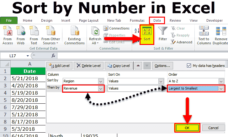
Step 3: Under "Sort by," select "Region" name. Under "Order," select A to Z.

Step 4: Click "Add Level" to add one more layer to the "Revenue" column.

Step 5: Under this layer, select "Revenue" first and then "Largest to Smallest."

Note: Firstly, Excel will sort region-wise data. Under this, it will sort revenue-wise from largest to smallest. By this sort, we easily get to know what is the highest revenue under each region.
Step 6: Click on "OK" to sort the data.

Things to Remember in Sort by Numbers in Excel
- We need to select the entire data range to sort. Otherwise, it will shuffle our data, and reports may go wrong.
- We need to click the checkbox: "My data has headers" to tell Excel not to consider the first row as data.
- We can use the numbers from smallest to largest and largest to smallest.
- In the case of non-numerical data, we can sort from A to Z, Z to A.
- We can sort dates from "Oldest to Newest," "Newest to Oldest."
- We can add many layers to alter the data according to our wishes.
- In the case of sorting based on the cell’s color or font color, we can sort only one color at a time. So, we would suggest you use it if required.

