Slicers In Excel

Last Updated :

Blog Author :

Edited by :

Reviewed by :

Download FREE Slicers Excel Template and Follow Along!

Slicers Excel Template.xlsx

Table Of Contents

What Do You Mean By Slicers In Excel?

Slicers are a useful Excel feature that uses multiple auto filters in a data table. However, if a user has to use the filter on every column to find a date, it involves many clicks, while inserting a slicer makes it easier for the user as few clicks can do it. Slicers are available in the “Insert” tab in the “Filters” option.

For example, consider the below table showing highest marks obtained by students in three semesters. Now, let us learn how to insert slicers and filter data easily.

Slicers in Excel Example - 1

Step 1: First, convert the data into a table. So, press Ctrl + T and click on My Table has headers option. Then, click OK.
Step 2: Next, we will be able to see Insert Slicer option under the Table Design tab.
Step 3: We can see the Insert Slicers window. We can select as many filters as we want and click OK. In this example, we have selected semesters.

Now, we can see semester window with 3 options – 1, 2 and 3. When we select 1, Excel will filter the table and show only semester 1 data as shown in the below image.

Slicers in Excel Example - 2

Likewise, we can use slicers in Excel.

Key Takeaways

The Slicers in Excel are used to filter the data effectively.
Remember, we can use slicers in Excel only when the data is converted into a table. We can convert data using the shortcut keys Ctrl +T.
We must select My Table has headers if our table has headers.
Using slicers in Excel, we can select multiple filters.
To multiselect slicers in Excel, simply use the shortcut keys Alt + S or press the multiselect option in the slicers window.

How To Use Slicer In Excel?

#1 - How To Insert Slicer To Your Regular Excel Table?

We can also insert a slicer into the Excel tables. Now, look at the below normal data range. You will not see any slicer option for this normal data range.

It would help if you converted the normal data range to Excel tables to unleash the option of slicers in Excel.

Below are the steps to insert a slicer into the regular Excel table:

First, select the entire data and press “Ctrl + T” to add a table to the data range.
Click on “OK.” It will create a table for you.
As soon as the table has been created, you will see a new tab in the ribbon called “Design.” Under this tab, you can see the “Slicers” option (only from Excel 2013 onwards).
Select the option of “Insert Slicer.” It will show you all the available headings in the table.
Select the required column you want to filter out the data quite often.
Note: You can select all the headings as well. But we have chosen the “Country” column heading only.

It is the slicer we have inserted for the heading “Country.” It will list out all the unique values from the list. Clicking on a specific country data table will display only the selected country’s data.

We have selected the country name “Canada,” and the data table shows only Canada’s data.

#2 - How To Insert A Slicer To Your Pivot Table?

We are sure you are smiling at slicers’ attractive options and cool features. However, do not be overwhelmed by the cool features of the slicer because we have a lot more in it to reveal many things. Note: download the workbook to follow here.

When we apply the PivotTable, which has many fields, it often fails to convey the correct message due to too many areas. We are sure you have also experienced this in your daily work. But inserting a slicer into the table makes the report more user-friendly.

We have a large data table with as many as 10 headings and more than 700 rows of data.

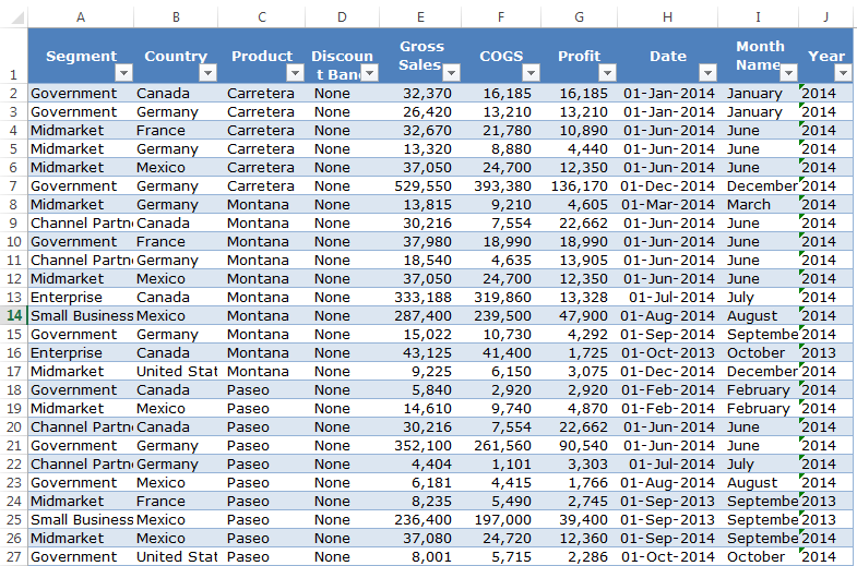
We want a summary of this large data regarding its gross sale. Therefore, we have applied the PivotTable to summarize this large data.

We want to see the summary report in terms of country-wise, product-wise, year-wise, and segment-wise.

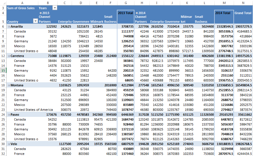
PivotTable showed us the summarized report because the data has many fields, and the report is not user-friendly as of now. However, by inserting a slicer, we can create user-friendly filter options.

Step 1: Place a cursor inside the pivot table. Remove all the fields except “Country” and “Years.”

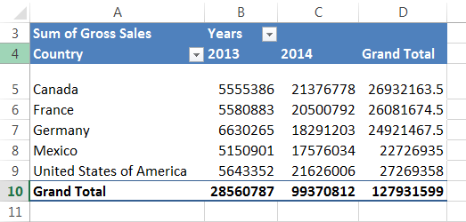
Step 2: Go to “Analyze” → “Insert Slicer.”

Step 3: Once the slicer is selected, it will show all the headings. Select “Segment” and “Product.”

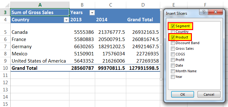
Step 4: Now, you will see the slicers for these two selected headings.

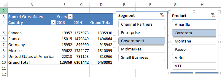
The report shows the summary of all the segments and all the products. If you wish to filter out the report only for the segment “Government” and the product “Carretera,” you can select the options from the slicers. The PivotTable begins to show the report only for the applied filters. Only “Government” and “Carretera” have been highlighted in the slicer.

#3 - How To Add Slicer For Two Pivot Tables

We can apply the same slicer for two PivotTables. For example, see the image below, where we have two PivotTables.

First, the pivot table shows the report segment-wise, and the second table shows the report country-wise. We need to analyze month-wise for both the PivotTables. We will insert a slicer for one first PivotTable as of now.

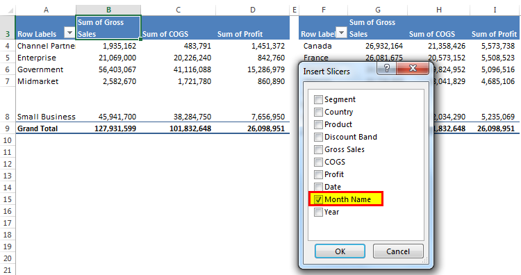
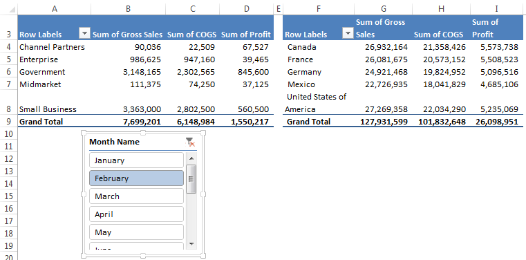
In the above image, we have selected February month as the filter. Therefore, the first PivotTable shows the result only for February. However, a second pivot table still leads the overall report for all the months.

To link the slicer with the PivotTables, right-click on “Slicer” and select the “Report Connections” option.

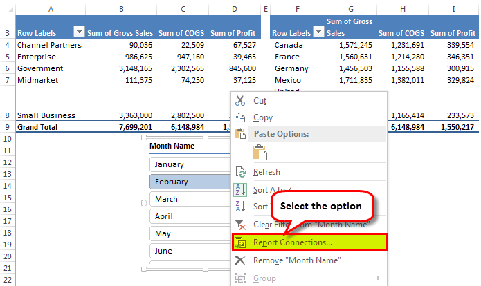
Once you click “Report Connections,” it will show you the list of the same data table’s all the PivotTables in the workbook. Next, select the number of PivotTables you need to link to this slicer. In this case, only two PivotTables.

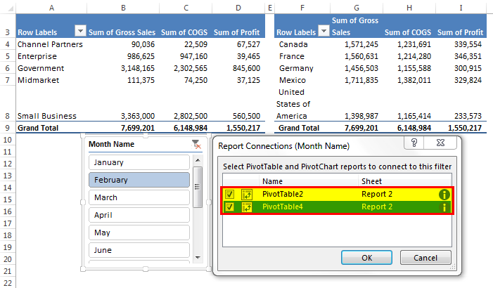
Now, return and select the month name you want to display in the report.

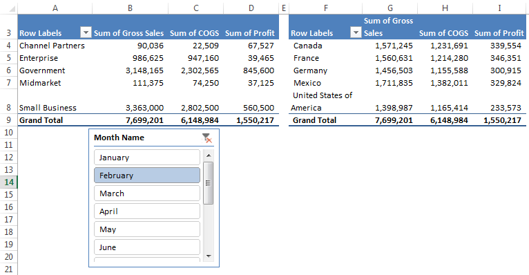
Now, both the PivotTables are showing the report for February only.

#4 - How To Adjust Slicer To Fit Your Window?

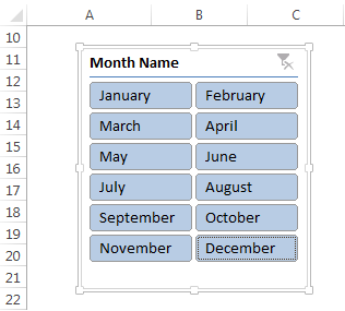
One of the common problems in SLICER is a spacing problem. Now, look at the below slicer table for MONTHS.

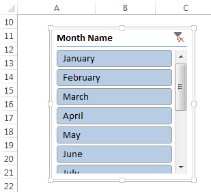
This slicer shows only the first six months in the present display. So, if we want to choose the remaining months, we need to scroll down and select, and it will take some time off my productivity. But we can make some alignment changes to display as per my convenience.

Step 1: Select the “Slicer” and go to “Options.”

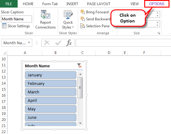
Step 2: Under this option, go to “Columns” and make it “2.”

Under this option, go to “Columns” and make it “2.”

Important Things To Note

In the case of linking PivotTables, we must be aware of PivotTable names. Therefore, it is always a better technique to give names to the PivotTables.
We can control the dashboards through slicers.
The slicer and PivotTables are interdependent.