Excel REPLACE Function

The REPLACE function in Excel is a text function that is an inbuilt function similar to a substitute function. This function replaces an old text from a string with a new string. The input required by this function is the old text, new text, the starting numbers, and ending numbers of the characters, which need to be replaced.

For example, suppose we have an Excel spreadsheet with numbers and text. We need to replace the number "517" with the other number "987" while retaining the text "ABC." Using the Excel REPLACE function, we can apply the formula below:

=REPLACE("ABC517",4,3,"987") returns "ABC987".

• The Excel REPLACE function is a Text function thathelps users replace an old text character or an entire string with a new set of characters or strings.
• As a worksheet function, it can be written as a part of a formula in a worksheet cell. It can be used in macro code as a VBA function, entered through the Microsoft Visual Basic Editor integrated with MS Excel.
• The second parameter, start_num, and the third parameter, num_chars, cannot have a non-numeric or a negative value.

The syntax of the Excel REPLACE formula is,

Where,

• old_text: This is a required parameter. It is the original string to be replaced.
• start_num: It is the starting position in the original string from where the replacement should begin.
• num_chars: It is a numeric value and indicates the number of characters to be replaced.
• new_text: It is another required parameter and indicates the new string/set of characters to be replaced the old_text with.

The REPLACE function is used in 2 ways, namely,

1. Access from the Excel ribbon.
2. Enter in the worksheet manually.

Method #1: Access from the Excel ribbon

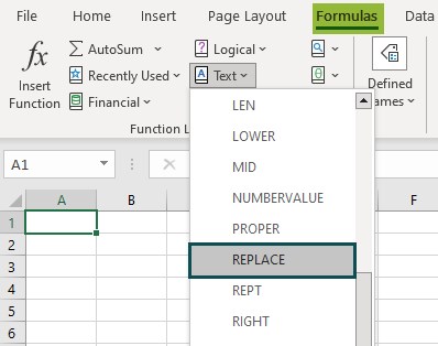
First, choose an empty cell - select the “Formulas” tab - go to the “Function Library” group - click the “Text” option drop-down - select the “REPLACE” function, as shown below.

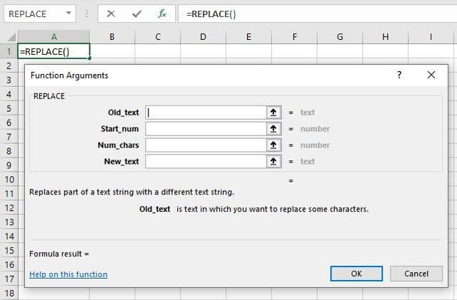
The “Function Arguments” window opens. Enter the arguments in the “Old_text, Start_num, Num_chars, New_text” fields, and click “OK”, as shown below.

Method #2: Enter in the worksheet manually

1. Choose an empty cell for the output.
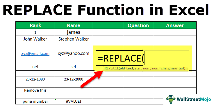
2. Type =REPLACE( in the cell.
3. Enter the arguments as cell values or cell references.
4. Close the brackets, and press the “Enter” key to execute the formula.

We will consider some specific scenarios and their corresponding examples, such as,

• Replace a string
• Replace a Substring
• Replace a Single Character
• Replace numbers
• Remove a string
• Common Problem with REPLACE function

Example #1 - Replace a string

In this example, cell C4 has a REPLACE formula associated with it. So, C4 is a result cell.

The old string is “John”, and the new string is “Stephen”.

Example #2 - Replace a Substring

In this example, cell C6 has a formula associated with it. So, C6 is a result cell.

• The first argument of the REPLACE function is B6, which contains the original string to be replaced.
• The second argument is 5, which indicates the starting letter of the original string.
• The third argument is 5, which is the number of characters to be replaced.
• The fourth and last parameter is yahoo, a new string to be replaced with.

The old string is “gmail”, and the new string is “yahoo”. As a result, C6 is updated with “xyz@yahoo.com.”

Example #3 - Replace a Single Character

In this example, cell C8 has a REPLACE formula associated with it. So, C8 is a result cell.

• The first argument of the REPLACE function is B8, which contains the original string to be replaced.
• The second argument is 1, which indicates the starting letter of the original string.
• The third argument is 1, which is the number of characters to be replaced.
• The fourth and last parameter is “s,” which is a new character to be replaced with.

Here, the old character is n, and the new character is s. As a result, C8 is updated with “set.”

Example #4 - Replace numbers

In this example, cell C10 has a REPLACE formula associated with it. So, C10 is a result cell.

• The first argument of the REPLACE function is B10, which contains the original string to be replaced.
• The second argument is 7, which indicates the starting letter of the original string.
• The third argument is 4, which is the number of characters to be replaced.
• The fourth and last parameter is “2000,” a new string to be returned with.

The old string is “1989.” The new string is “2000.” As a result, C8 is updated with “23-12-2000.”

Example #5 - Remove a string

In this example, cell C12 has a REPLACE formula associated with it. So, C12 is a result cell.

• The first argument of the REPLACE function is B12, which contains the original string to be replaced.
• The second argument is 1, which indicates the starting letter of the original string.
• The third argument is 11, which is the number of characters to be replaced.
• The fourth and last parameter is "" which is a new string (an empty string) to be replaced with.

Here, the old string is “Remove this,” and the new string is “”. As a result, C12 is updated to a blank cell as all the characters are replaced with blanks.

Example #6 - Common Problem with REPLACE Function

In this example, cell C14 has a REPLACE formula associated with it. So, C14 is a result cell.

• The first argument of the REPLACE function is B14, which contains the original string to be replaced.
• The second argument is 0.

However, any string in an Excel worksheet cell starts with 1, index 1. So, the result in cell C14 is an error which is #VALUE! indicating that there is an error in the value.

• We get the #VALUE! error, when either of the second, third, or fourth argument value is not provided.
• If the proper cell value or cell reference is not selected, we get the “#NAME?” error.

This article must help understand Excel REPLACE function with its formulas and examples. You can download the template here to use it instantly.

This article has been a guide to Excel REPLACE Function. Here we replace/substitute existing string/text with another string, examples & downloadable excel template. You may also look at these useful functions in Excel: -

• Excel VBA Find and Replace
• VBA Replace String
• Substring Function in VBA
• Left Function in VBA | Examples
• Excel MAXIFS