Remove Duplicates From Excel Column

Publication Date :

24 Apr, 2019

Blog Author :

Edited by :

Reviewed by :

Download FREE Remove Duplicates From Column Excel Template and Follow Along!

Excel Column Remove Duplicates.xlsx

Table Of Contents

What Is Remove Duplicates From Excel Column?

Remove duplicates from excel column is a method used to remove duplicate entries in the data, column-wise. We can easily remove duplicates in Excel using 3 methods.

For example, consider the below table showing student’s names. Now, let us remove the duplicates in the column.

Remove Duplicates from Excel Column - Intro.jpg

Step 1: First, select the column where we want to remove duplicates. In this example, select column A.

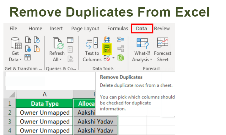
Step 2: Next, select Data - Remove Duplicates under the Data Tools group.

Step 3: Now, select Continue with the current selection in the Remove Duplicates Warning window. Then, click Remove Duplicates.

Step 4: In the following Remove Duplicates window, make sure the column we want to remove duplicates is selected and click OK.

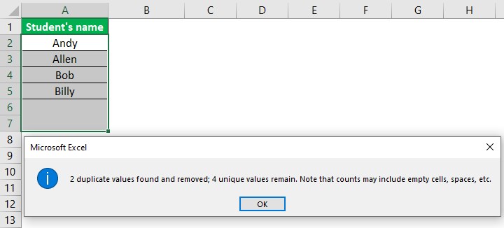
We will see a pop-up showing that Excel has removed the number of duplicates as shown in the following image.

Remove Duplicates from Excel Column - Intro - Output.jpg

Likewise, we can remove duplicates in Excel.

Key Takeaways

Remove duplicates from excel column method helps users remove duplicate entries in the selected column.
To remove duplicate entries in Excel, users can use any of the three methods. They are:
Using Data Tools group. Using Advanced Filter in Excel Conditional formatting in Excel
Remember, while removing duplicates using data tools group, simply select the column where we want to remove the duplicates and click on Data > Remove Duplicates under the Data Tools group in Excel.

How To Remove Duplicates In Excel? (Top 3 Methods)

Using Data Tools group.
Using Advanced Filter in Excel
Conditional formatting in Excel

We will learn all three methods of Excel column removing duplicates by a few examples.

#1 - Remove Duplicates From Data Tools Group

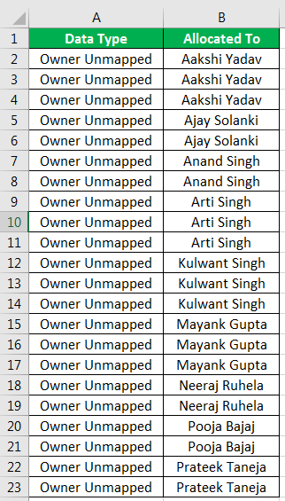
Suppose we have data in our sheet as below.

We want to check how many people’s names are mentioned in column B. We can count the number of unique names for a smaller amount of data. But it may take a while to figure out the same for a larger amount of data. It is where removing duplicates in Excel comes in handy.

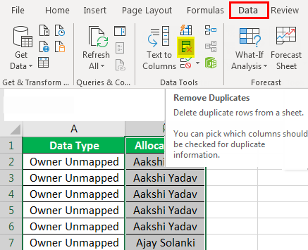
Select column B. In the “Data” tab, under the “Data Tools” section, click on “Remove Duplicates.”
A dialog box appears. It asks if we want to remove duplicates from the current selection or if we want to expand our selection. As column A has just one type of data, and we need to remove duplicates from column B, we will select “Continue with the current selection.”
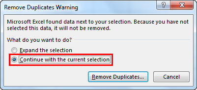
After selecting, “Continue with the current selection,” click on “Remove Duplicates,” another dialog box appears.
It tells us to select the column from which we want to remove duplicates. If we had chosen the whole data, it would show all the columns, and it is up to us to determine the column from which we want to remove duplicates.
As column B is selected, we click on “OK,” and Excel prompts us that the duplicated data has been deleted and only the unique values remain.
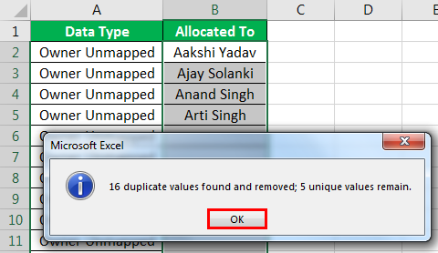
We can see that the duplicate data has been deleted from column B, and only the unique values remain.

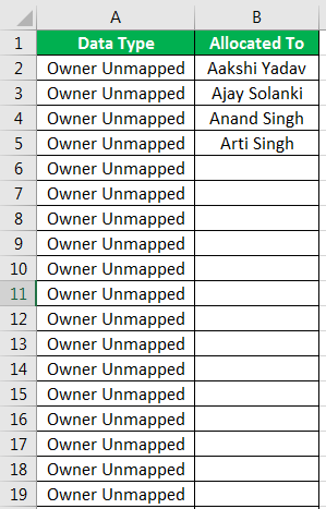
The above method was the first method of removing duplicates.

#2 - Using Advanced Filter In Excel

Now, we will try to remove duplicate data from the "advanced filter" tool.

Let us consider the same data in sheet 2 and try to delete the duplicate data using the second method.

The data is the same as below,

Step 1 - Under the same “Data” tab, in the “Sort & Filter” section, click on “Advanced Filters.” A dialog box appears.

Step 2 - Select "Copy to another location."

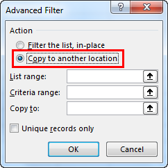
Step 3 - We need to provide the data range to the advanced filter so we can select our data in the sheet.

Step 4 - In the “Copy to:” box, we must give a location where the data needs to copy. For the current scenario, we will choose a location in the current sheet. We can choose any other sheet also.

Step 5 - Now, select “Unique records only,” as it will filter out the duplicate data and paste only the unique data to the new destination.

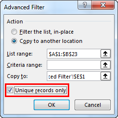
Step 6 - When we click on “OK,” we can see that the data has been pasted to the destination. However, there are no duplicate values.

The above method was the second method of removing duplicates using the advanced filter tool.

#3 - Conditional Formatting To Remove Excel Column Duplicates

Now, we will use the third option, the conditional formatting method.

Consider the following data for the example.

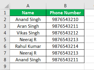
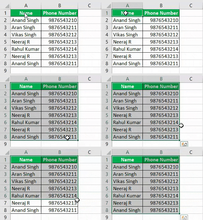
Step 1 - Select the data in the sheet.

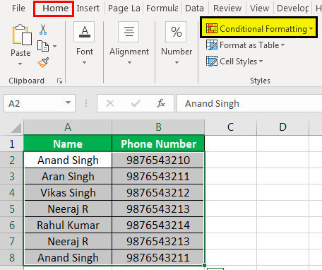
Step 2 - Now, in the “Home” tab under the “Styles” section, click on “Conditional Formatting.”

Step 3 - A dialog box appears. In the “Highlight Cells Rules,” click on “Duplicate Values.”

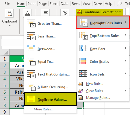
Step 4 - Another dialog box pops up. Again, Excel automatically highlights the values which are duplicates.

Step 5 - Click on “OK.” Now, we can see how much our data is duplicated. There are four duplicate data.

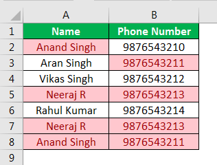
We can now remove the duplicate data.

Important Things To Note

Removing duplicates in the “Data Tools” option keeps the first value and removes the other duplicates.
The same is with the second method. It also removes duplicate data, and the first one is considered unique.
The conditional formatting method helps to see how much data is duplicated.