Remove (Delete) Blank Rows in Excel

Last Updated :

Blog Author :

Edited by :

Reviewed by :

Table Of Contents

Removing Blank Rows in Excel

Removing blank rows implies deleting the empty rows of an Excel worksheet. An empty (or blank) row is one that does not contain any data values. Such blank rows can cause errors in the applied formulas and make the excel dataset look unorganized and untidy.

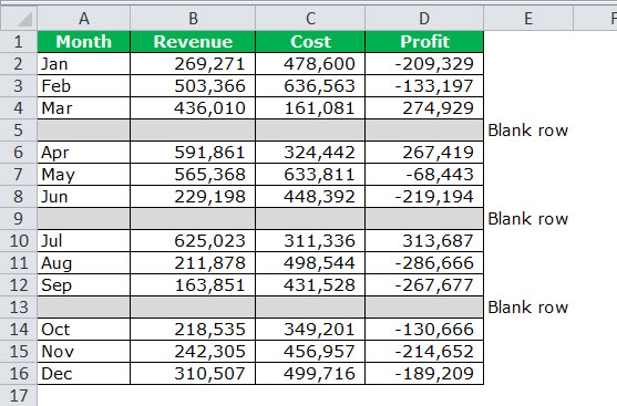
For example, some unwanted data was removed from row 4 of the following excel dataset. This deletion has created a vacuum in the worksheet, suggesting incomplete or missing entries. Hence, it is essential to eliminate such blank rows from the dataset.

Blank rows appear in a worksheet due to different reasons like copying data from another database, importing data from the Internet, receiving data from other team members, and so on. The purpose of deleting blank rows is to deliver clean datasets that are fit for further processing and analysis.

This article discusses the different techniques for removing (deleting) blank rows in Excel.

Removing Blank Rows in Excel
How to Remove (Delete) Blank Rows in Excel?

How to Remove (Delete) Blank Rows in Excel?

The techniques of removing blank rows from an Excel worksheet are listed as follows:

Manual deletion
Deletion using the “go to special” window
Deletion using filters
Deletion using the COUNT function

Let us explore these methods one by one with the help of examples.

#1–Manual Deletion of Blank Rows in Excel

This method is quite helpful when the dataset is small. Moreover, it is an easy technique that does not take much time when applied.

Example #1

The following image shows the revenues generated (column B), costs incurred (column C), and profits earned (column D) by an organization for the different months (column A). The negative figures of column D represent losses.

The dataset pertains to the year 2016. Further, there are three blank excel rows in this dataset, which we want to delete using the following methods:

“Delete sheet rows” option of the Home tab
“Delete” option of the context menu
“Ctrl+minus (-)” shortcut

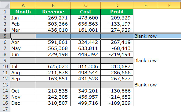
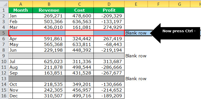
Step 1: Select the first blank row (row 5) of the dataset. For this, select any cell of row 5 and press the keys “Shift+space” together.

The selection is shown in the succeeding image.

Note: “Shift+space” is the shortcut key to select the entire row of the worksheet.

Step 2: Once the entire row has been selected, use any of the following methods to remove (delete) the blank Excel row:

Method “a”: From the Home tab, click the drop-down arrow of “delete” from the “cells” group. Next, select “delete sheet rows,” as shown in the following image.

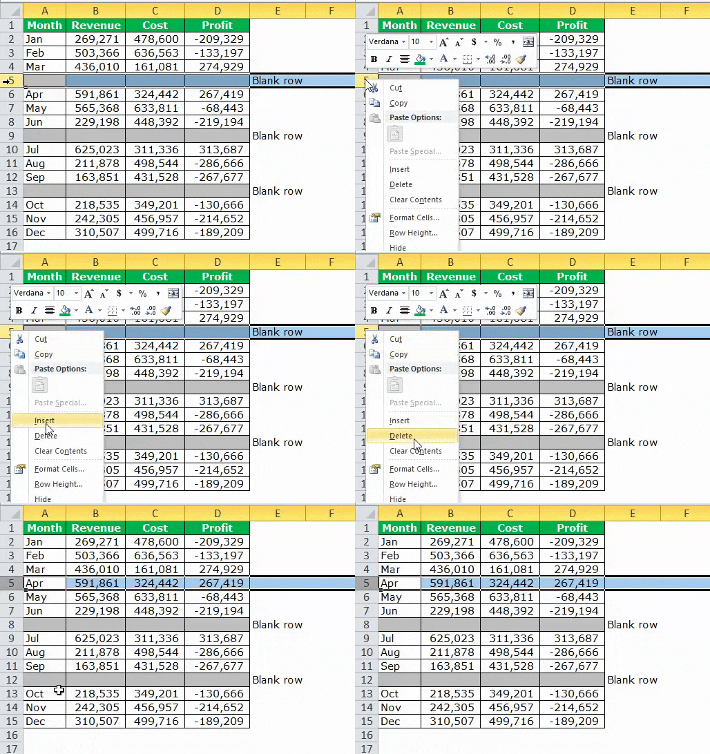
Method “b”: Right-click the selected row (row 5) and choose “delete” from the context menu. This is shown in the following image.

Method “c”: Press the keys “Ctrl+minus (-)” together. Had we selected a cell of row 5 rather than the entire row (in step 1), the “delete” dialog box would have opened. Next, one could have selected “entire row” and clicked “Ok.”

Note: “Ctrl+minus (-)” is the keyboard shortcut to delete the selected row or column entirely. For this shortcut to work, it is essential to select the row or column to be deleted in the foremost step.

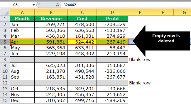
Step 3: The selected row (row 5 selected in step 1) is deleted. Consequently, the data of the initial rows 6, 7, and 8 has shifted upwards to rows 5, 6, and 7.

Hence, the vacuum at row 5 of the dataset has been filled up. This is shown in the following image.

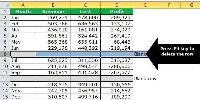
Step 4: Select the next blank row, which is row 8 of the current dataset. Next, press the F4 key to delete this selected row in excel.

The selected row is shown in the following image.

Note: The F4 key repeats the last action performed by the user. In this example, the last action performed was the deletion of the entire row 5.

In this way, all the blank rows of the given dataset are deleted. Hence, the size of the dataset has been reduced by eliminating unwanted rows.

#2–Deletion of Blank Rows Using the “Go To Special” Window of Excel

This method works well when a large number of rows have to be deleted from the dataset. In this technique, the blank rows are searched prior to being deleted.

Example #2

The following image shows a dataset similar to that of example 1. Notice that this time, the respective years have been added in column B. Moreover, the data for 2017 has also been added in the bottom rows.

We want to delete all the blank excel rows with the help of the “go to special” dialog box.

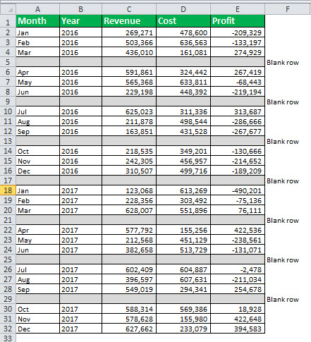
The steps to remove the blank rows in excel using the given technique are listed as follows:

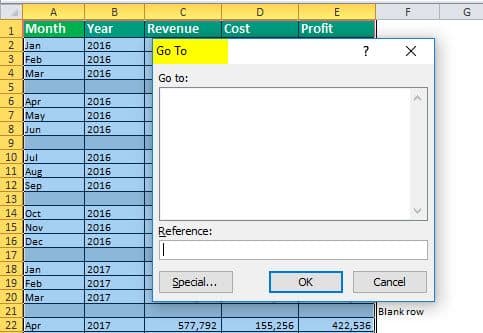
Select the entire dataset. Next, press the keys “Ctrl+G” together. The “go to” dialog box opens, as shown in the following image.

Note: The shortcut “Ctrl+G” opens the “go to” window of Excel.
Click “special,” shown within a red box in the following image. Alternatively, one can press the keys “Alt+S.”
The “go to special” dialog box opens. Choose “blanks” or press the key “K” and click “Ok.” The selection of this option is shown in the following image.

Note: Another way to access the “go to special” dialog box is to click the “find and select” drop-down from the Home tab. Thereafter, select the option “go to special.”
All blanks within the selected region (selected in step 1) are highlighted. This is shown in the following image.
Keep cell A5 selected. This is the first blank cell that was selected by the “go to special” window in the preceding step.

Press the keys “Ctrl+minus (-)” together. The “delete” box opens, as shown in the following image. From this box, select “entire row” and click “Ok.”
All the blank rows are deleted, as shown in the following image. The data values shift upwards and fill up the blank rows that had existed initially.

The current dataset consists of 25 rows as against the previous one (shown at the start of this example), which had 32 rows. Hence, this cleaned dataset offers an improved display to the user.

#3–Deletion of Blank Rows Using Filters in Excel

In this method, the blank rows are filtered, selected, and deleted.

Example #3

Working on the data of example #2, we want to remove the blank excel rows by filtering them.

The steps for the given task are listed as follows:

Step 1: Select the entire dataset (or the entire worksheet) and add excel filters. For adding filters, click the “sort and filter” drop-down from the “editing” group of the Home tab. Next, choose “filter.”

Alternatively, select “filter” from the “sort and filter” group of the Data tab. The filters have been added to the dataset, as shown in the following image.

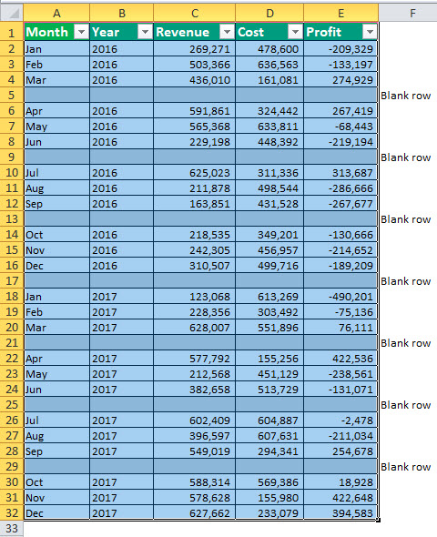
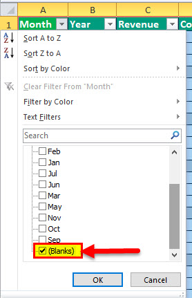
Step 2: Click the filter of “month.” Uncheck the “select all” option to deselect all the months. Select “blanks,” as shown in the following image. Next, click “Ok.”

Note: Be careful while selecting the blank cells since these will be deleted in the subsequent steps. Ensure that no data cells are selected.

Step 3: At present, only the blank rows of the dataset are visible. These are shown in the following image.

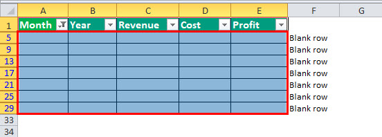
Step 4: Select all the filtered rows. Ensure that the top row containing the column headers is not selected. Next, press the keys “Alt+semicolon (;)” together. For this, hold the “Alt” key and, at the same time, press the semicolon.

The visible blank cells are selected, as shown in the following image.

Note: “Alt+semicolon (;)” is the shortcut to select only the visible cells of a selection. It ignores the hidden rows and columns of the selection.

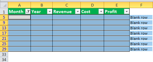
Step 5: Once the visible cells are selected, press the keys “Ctrl+minus sign (-)” together. If a warning appears, which asks if the entire sheet row has to be deleted, click “Ok.”

Step 6: All the blank excel rows are deleted from the given dataset. In the filter of “month,” check the “select all” option to view the entire dataset. Clear the filters by clicking the “filter” option (or the “clear” option) from the Home tab or the Data tab.

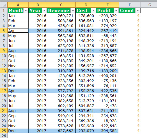
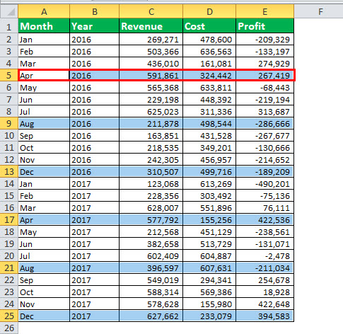
Hence, the cleaned dataset is shown in the following image. The rows appearing in blue were earlier blank. But, now they have been filled by an upward movement of the data values.

#4–Deletion of Blank Rows Using the COUNT Function of Excel

In this method, the COUNT function is applied to filter and delete blank rows.

Example #4

Working on the data of example #2, we want to remove the blank rows by applying the COUNT excel formula. The rows which return zero (0) as the result of the COUNT formula should be filtered and deleted.

The steps for removing blank rows by applying the COUNT formula are given as follows:

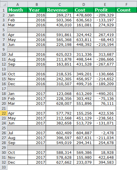
Step 1: Insert a new column (column F) titled “count.” This is shown in the following image.

Step 2: Enter the following COUNT formula in cell F2.

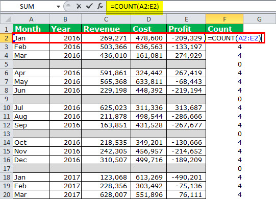
“=COUNT(A2:E2)”

Press the “Enter” key. To obtain the outputs for the entire column F, drag the formula of cell F2 till the last data cell of column F.

The results are shown in the following image. For all the blank rows, the COUNT formula returns zero. For the remaining rows, this formula returns the count of numerical cells.

Note: The COUNT formula counts the number of cells containing numerical values in the given range (like A2:E2). If no numerical values are found in a particular range, the formula returns zero.

Step 3: Add filters to the dataset (refer to step 1 of example #3). Click the filter of the “count” column. Deselect option four (4) and select option zero (0). This is shown in the following image.

Click “Ok” once the required checkbox is selected.

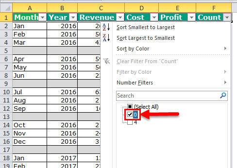
Step 4: The dataset shows those rows for which the COUNT formula has returned zero. Select these filtered rows, which show 0 in column F. Press the keys “Alt+semicolon (;)” to select the visible cells.

The selection is shown in the following image. Next, press the shortcut “Ctrl+minus (-)” to delete these blank rows. If a warning is displayed asking whether the entire row should be deleted, click “Ok.”

Step 5: The blank rows have been deleted. From the filter of the “count” column, check the “select all” option. The cleaned dataset is shown in the following image.

We have not removed the filters though one can remove them if required. The column “count” can also be deleted since it has met the goal of eliminating blank rows from the dataset.

Frequently Asked Questions

1. What does it mean to remove blank rows in Excel?

To remove blank rows implies deleting the empty rows of an exceldataset. These rows are usually not required as their presence makes the dataset look disordered. Moreover, they make navigation within the worksheet difficult.

In Excel, there are several techniques for removing blank rows. This article discusses all these methods with the help of examples. One can follow the technique, which is easy and quick to be applied.

Note: For more details about the different methods, refer to the examples of this article.

2. How to remove the blank rows displayed at the bottom of the Excel worksheet?

It is not possible to delete the blank rows displayed at the bottom of the worksheet. However, hiding such rows is possible. The steps for the same are listed as follows:

a. Select a cell of the first blank row to be hidden.
b. Press the keys “Shift+space” together. This selects the entire row.
c. Press the keys “Ctrl+Shift+down arrow” together. This selects till the last blank row of the current worksheet.
d. Right-click any row number of the selection.
e. Choose “hide” from the context menu.

All the blank rows displayed at the bottom of the worksheet will be hidden. Such hidden rows are present in the worksheet even though they are invisible.

Note: To unhide the hidden blank rows, select the worksheet by pressing the keys “Ctrl+A” together. Right-click the selection and choose “unhide” from the context menu.

3. How to remove blank rows by using a formula in Excel?

The steps to remove blank rows by using an Excel formula are listed as follows:

a. Add a column to the dataset. Label it “helper” as it serves as a helper column. This column should be adjacent to the data columns of the worksheet.
b. Enter the formula “=COUNTBLANK(range)” in the first cell of the helper column. For instance, if the range is A2:D2, type the formula as “=COUNTBLANK(A2:D2).”
c. Press the “Enter” key and drag the formula to the remaining cells of the helper column.
d. Add filters to the dataset by clicking the filter icon in the Home tab (“editing” group) or the Data tab (“sort and filter” group).
e. Deselect the option “select all” from the filter of the helper column. Select the checkbox of the maximum number displayed. Suppose, for the range A2:D2, the maximum output returned by the COUNTBLANK is 4. This implies that all four cells (from A2 to D2) in row 2 are empty.
f. Select the filtered rows, which show the maximum output (like 4) of the COUNTBLANK function. Right-click the selection and choose “delete row” from the context menu.
g. Click “Ok” in the message asking if the entire row is to be deleted.
The blank rows have been eliminated from the dataset. To view the complete dataset (excluding the blank rows), check the option “select all” from the filter of the helper column. One can clear filters and delete the helper column if required.

Note 1: A helper column is a supporting column added to the dataset to simplify calculations.

Note 2: The COUNTBLANK formula counts the number of empty cells within the specified range. In step b, we specified the range as A2:D2. So, the COUNTBLANK counts empty cells in row 2, which begins from cell A2 and ends at cell D2.