Rate Function in Excel

Last Updated :

Blog Author :

Edited by :

Reviewed by :

Table Of Contents

RATE Excel Function

The RATE function in Excel is used to calculate the rate levied on a period of a loan. It is a built-in function in Excel. It takes the number of payment periods, pmt, present value, and future value as an input. The input provided to this formula is in integers, and the output is in percentages.

For example, suppose we have a dataset of the 5-year loan of $25,000 in cell B1 with monthly payments of $1000 in cell B2 has 60 periods in cell B3. We need to find the interest rate on the student loan. In such a scenario, we can use the RATE function in Excel:

=RATE(B3,B2,-B1)*12

=4.1%.

RATE Excel Function

RATE Formula in Excel

Explanation

Compulsory Parameter:

Nper: Nper is the total number of the period for the loan/investment amount to be paid. For example, considering the 5 years terms means 5*12=60.
Pmt: The fixed amount paid per period cannot be changed during the annuity's life.
Pv: Pv is the total loan amount or present value.

Optional Parameter:

: It is also called the future value and is optional in the RATE function in Excel. And if not passed in this function, it will be considered zero.
: It can be omitted from the RATE function in Excel and used as 1 if payments are due at the beginning of the period and considered as 0 in case the payments are due at the end of the period.
: It is also an optional parameter; if omitted, it is assumed as 10%.

How to Use the RATE Function in Excel?

The RATE function in Excel is very simple and easy to use and can be used as a worksheet function and VBA function. Therefore, this function is used as a worksheet function.

Example #1

Suppose the investment amount is 25,000, and the period is 5 years. Here the number of payments nper will be =5*12=60 payments in total, and we have considered 500 as a fixed monthly payment and then calculated the interest rate using the RATE function in Excel.

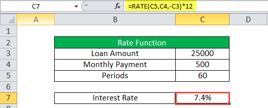
Output will be: =RATE (C5, C4,-C3)*12 = 7.4%

Example #2

Let us consider another example wherein the interest rate per payment period on a 5,000 investment amount where monthly payments of 250 are made for 2 years so period will be=12*2=24. Here we have considered that all payments are made at the beginning of the period, so the type will be 1.

Calculation of interest rate are as follows:

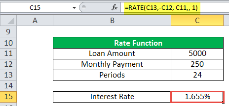
=RATE(C13,-C12, C11,, 1) output will be: 1.655%

Example #3

Let us take another example for weekly payment. This next example returns the interest rate on a loan amount of 8,000 where weekly payments of 700 are made for 4 years. Here, we have considered that all payments are made at the end of the period so that type will be 0 here.

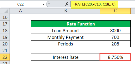
The output will be: =RATE(C20,-C19, C18,, 0) = 8.750%.

Example #4

In the final example, we have considered that the loan amount will be 8,000, and annual payments of 950 are made for 10 years. Here, we assume that all the payments are made at the end of the period, then the type will be 0.

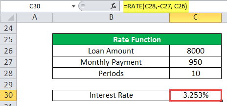
The output will be: =RATE(C28,-C27, C26) =3.253%

RATE in Excel is used as a VBA function.

Dim Rate_value As Double

Rate_value = Rate(10*1, -950, 800)

Msgbox Rate_value

And output will be 0.3253

Things to Remember

Below are the few error details that can come in RATE in Excel if wrong arguments are passed in the RATE function in Excel.

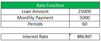
Error handling #NUM!: If the interest RATE does not converge to 0.0000001 after 20 iterations, then the RATE excel function returns the #NUM! Error value.

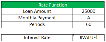
Error handling #VALUE!: The RATE Excel function through a #VALUE! Error when any non-numeric value has been passed in the RATE formula in the Excel argument.

We must convert the number of periods to month or quarter per your requirement.
If the output of this function seems like 0, then there is no decimal value, then we must format the cell value to percentage format.