Table Of Contents
Excel RANK Function
Excel RANK formula is used to give us the rank of a given dataset of numbers based on the data set, or we can say by comparing the other numbers in the data set. The RANK function was a built-in function for Excel 2007 and earlier versions. For newer versions above 2007, we have a built-in function as RANK.Avg and RANK.Eq functions.
For example, suppose there is a list of students' scores in cells C2:C10. Then, we can use the RANK function in Excel to find the student's rank.
The RANK function is a built-in function in MS Excel. It falls under the category of STATISTICAL functions in Excel. This function is used to get the rank of a given number from the list of numbers.
Syntax

The RANK formula in Excel has three arguments: the first two are required, and the last one is optional.
- number = A number for which the rank is to be found out.
- ref = the range of numbers concerning which the rank of a given number is to be found.
- order = the order (ascending or descending) in which we should rank the numbers. 0 = Descending order; 1 = Ascending order. If the order is omitted, the default value is zero, i.e., descending order.
How to Use RANK Function in Excel? (with Examples)
The given function is a WorkSheet (WS) function. As a worksheet function, it can be entered as a part of the formula in a worksheet cell. Refer to the examples explained in this article as you proceed to learn more.
Example #1 - Find Steve’s Rank in Maths

- The above example shows the students' marks in Maths and Science subjects. We would use the Excel RANK function to find Steve’s rank in Maths.
- The first parameter is the input value, of which the rank is to be calculated. Here, B6 represents Steve’s marks in Maths, 68.
- The total cells containing Maths marks are the second parameter from B1 to B11. So, the range is B1:B11, which comprises all students’ marks in Maths.

- The highest value represents the rank 1, and the lowest represents the last rank. So, the third parameter is skipped, and Excel treats it as 0. The default order is descending.
- The RANK (B6, B1: B11) function returns the rank of the student named Steve in the subject Maths as 8, 50 being the lowest (B2) and 99 (B10) being the highest marks in Maths subject.

Example #2 - Find the Lowest Runtime from the Race Record

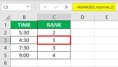
- In the above example, different time values are given. We have to find the lowest runtime from the provided records.
- The time values range from cell B1:B6. So, the cell range is named as a table and called "my time." It acts as an alias for B1: B6.

- Unlike example #1, the lowest runtime indicates the 1st rank, and the highest runtime indicates the last rank. So, we need to apply ascending order while calculating the rank in Excel. Hence, the third parameter is given as 1.
- So, the RANK (B3, my time, 1) function returns the lowest runtime as the rank 1 from the given race times.

- As a result, at 4:30 (cell B3), the lowest one is recorded as rank 1, and at 9:00 (cell B5), the longest one is recorded as the last, i.e., the 4th rank.
Example #3 - Value Not Present

- As shown in the above figure, the first parameter, which is the value for which the rank is to be calculated, is NOT present in the range of cells given in the second parameter, then the Excel RANK formula returns #NA! Error indicating that the value is invalid, i.e., not present in the given range of reference cells.
- As shown in the above figure, number 59 is not in the range. Hence, the #NA! Error is returned as a result shown in cell C8.
- One must correct the first parameter in such a case.
Example #4 - Text Formatted Numerical Values

- The first parameter, the value for which the rank is calculated, is given in the text format, “5,” as shown in the above figure. The value is not a number as it is quoted in double quotes. Hence, treated as a text.
- Since the rank cannot be calculated over text data, the function returns #N/A! The error indicates that the value is unavailable in the given range of cells. The resultant cell C6 has #N/A returned as the result of the function.

- One must correct the first parameter in such a case.
Things to Remember
- The minimal parameter the Excel RANK function takes is 2.
- The third parameter of the RANK function is optional and zero (descending order) by default. However, if specified as 1, the function treats it as ascending order.
- There is no RANKIF formula to perform a conditional ranking similar to COUNTIF in Excel. It needs the usage of an additional Excel function to achieve the same.
- When the given number for which the rank is to be calculated (first parameter) is not present in the range of cells provided as a reference to the function (second parameter), then #N/A! error occurs.
- The rank formula does not support any text values or the text representation of the numeric values as we cannot apply the RANK to text data. If provided, this Excel function returns the #N/A error, as explained.

