RAND Excel Function

The Random or RAND Excel function generates random values greater than 0 but less than 1. The distribution is even among those numbers if used on multiple cells. Every time we open the worksheet or refresh the formula, the result changes.

For example, when we type =RAND(), it generates a number like 0.902158.

RAND Excel Formula

The syntax of the RAND Excel Formula is,

The RAND formula in Excel has no parameters or arguments.

Explanation of the RAND Excel Function

• The RAND function is categorized as the “Math & Trig” function in Excel.
• It returns a random number between 0 and 1.
• The RAND function in Excel will generate a new random number greater than or equal to 0 and less than 1, each time your Excel sheet is refreshed.

The RAND In Excel function is very simple and easy to use.

• We can insert the formula from the “Formulas” tab from the “Math & Trig” group.
• We can enter in the worksheet manually as =RAND(), and
• We can use it as a VBA function.

RAND Excel Function As A Worksheet Function

The ways to enter the RAND function in the worksheet directly are as follows:

• One way, type =RAND() in an empty cell, press the “Enter” key to execute the formula, and return the generated result.

Or

• Alternatively, type =R or =RA, select the RAND function from the suggestions given by Excel, close the brackets , press the “Enter” key to execute the formula, and return the generated result.

We will consider some advanced scenarios using the RAND Excel function examples.

Example #1

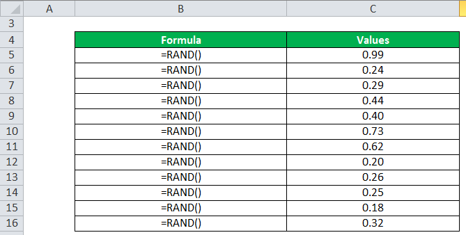
Let us consider the RAND() function to calculate the random numbers between 0 and 1. Then, the RAND Excel function returns the random numbers between 0 and 1, as shown in the table below.

Example #2

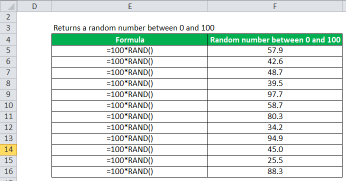
As you know, the RAND formula in Excel generates random numbers between 0 and 1. However, we can also return random numbers between 0 and 100, or any given range.

Ex. In the formula =100*RAND(),

• The RAND(), by default, generates random numbers Excel between 0 and 1.
• Then, the output is multiplied by 100 to get the digits between 0 and 100.

Finally, it will generate the random number in Excel, as shown below.

Example #3

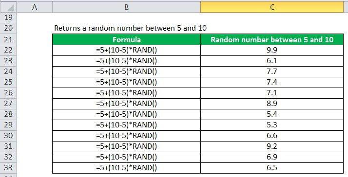
If you want to calculate the random number in Excel between two numbers, then we can use the RAND formula =a+ (b-a)*RAND(), where a and b may be any numbers.

The RAND formula generates the random number between two integers.

Therefore, the formula for the Random number formula in excel between 5 and 10 using will be,

 =5 + (10 – 5) * RAND().

Example #4

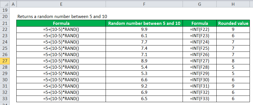
As considered in the Example 3, to generate the random numbers between 5 and 10, we used the RAND() formula =5 + (10 – 5) * RAND(), and generated random numbers between 5 and 10. Now, apply the INT() function to round the output integer to the output’s nearest positive integer, as shown.

Example #5

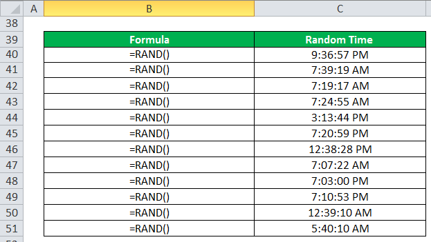
The RAND function also generates random time. So, let us apply RAND(), and then change the cell format to time.

Excel RAND Function As A VBA Function

To use the RAND Excel function as a VBA Function, we enter the following VBA Code in the VBAEditor module window.

Dim RandomNumber As Integer

RandomNumber = Int ((100 – 50 + 1) * Rnd + 50)

End Sub

In this example, the variable called RandomNumber would now contain a random number between 50 and 100.

• The RAND() function calculates a new value each time the worksheet is calculated. To overcome this problem,
  • We must convert the generated value to direct cell values.
  • We can copy the generated numbers and paste it in any other cells. Then the numbers will remain as constant.
• Also, to stop the auto change of the RAND() value, we must go to the go-to RAND formula Excel bar, and press F9 to convert the RAND formula in Excel into its result.
• We will get the “#NAME?” error, if we enter any cell values or cell references within the RAND() formula’s brackets. The function itself is a formula.