Product Excel Function

Last Updated :

Blog Author :

Edited by :

Reviewed by :

Table Of Contents

Product In Excel

The PRODUCT Excel function is a built-in mathematical function used to calculate the product or multiplication of the given number provided to this function as arguments. For example, if we give the formula arguments 2 and 3 as =PRODUCT(2,3), the result is 6. This function multiplies all the arguments.

The PRODUCT function in Excel takes the arguments (input as numbers) and gives the product (multiplication) as an output. So, for example, if cells A2 and A3 contain numbers, then we can multiply those numbers using PRODUCT in Excel.

Product In Excel

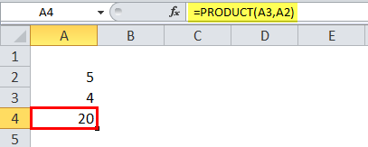
PRODUCT Formula in Excel

=PRODUCT(number1, , , ,….)

Explanation

The Excel PRODUCT formula has at least one argument. All other arguments are optional. Whenever we pass a single input number, it returns the value as 1*number, the number itself. The PRODUCT function in Excel is categorized as a Math/Trigonometric function. This PRODUCT formula in Excel can take up to 255 arguments in the later version after Excel 2003. In the Excel version 2003, the argument was limited to only 30 arguments.

The PRODUCT formula in Excel not only takes the input number one by one as an argument but also can take a range and return the product. So, if we have a range of values with numbers and want their product, we can do it by multiplying each one or directly using the PRODUCT formula in Excel, bypassing the value range.

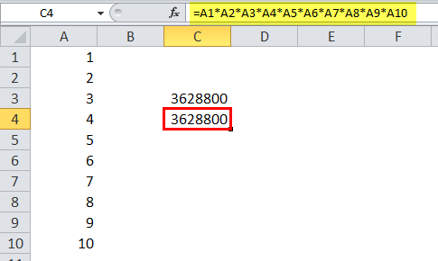
In the above figure, we want to multiply all the values in the range A1:A10. Suppose we use the multiply (*) mathematical operator, it will take much time compared to achieving the same using the PRODUCT function in Excel since we will have to select each value and multiply. Whereas using the PRODUCT function in Excel, we can pass the values directly as a range, and it will give the output.

=PRODUCT(A1:A10)

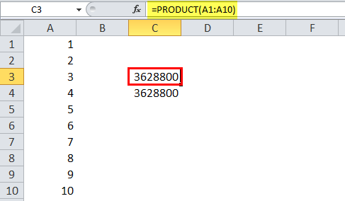
Therefore, the PRODUCT formula in Excel. =PRODUCT(A1:A10) is equivalent to the formula =A1*A2*A3*A4*A5*A6*A7*A8*A9*A10.

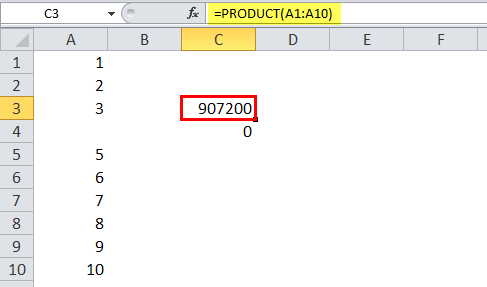
However, the only difference is when we use the PRODUCT function in Excel. If we leave the cell empty, PRODUCT in Excel takes the blank cell with the value 1 but uses the multiply operator. Therefore, Excel will take the value as 0. So, the result would be 0.

When we delete the cell value of A4, Excel considers it as a 0 and returns the output 0, as shown above. But, when we used the PRODUCT function in Excel, it took the input range A1:A10. The PRODUCT function in Excel seems to ignore cell A4, which was empty. However, it does not ignore the empty cell value but takes the blank cell with the value 1. It takes range A1:A10, considers the A4 with value 1, and multiplies the cells' values. Moreover, it also ignores text values and logical values. The PRODUCT function in Excel considers the dates and numeric values as numbers. Each argument can be supplied as a single value, cell reference, or an array of values or cells.

For small mathematical calculations, we can use the multiplication operator. Still, if we have to deal with a large data set where the multiplication of multiple values is involved, then this PRODUCT function serves a great purpose.

So, the PRODUCT function in Excel is beneficial when we need to multiply many numbers together, given in a range.

Examples

Let us look below are examples of the PRODUCT function in Excel. These Excel PRODUCT function examples will help you explore using the PRODUCT function in Excel.

Example #1

Suppose we have a set of values in columns A and B that contains numeric values with some empty cells. We want to multiply each value of column A with column B in such a manner that if any of the cells have an empty value, we get an empty value. Else, returns the product of two values.

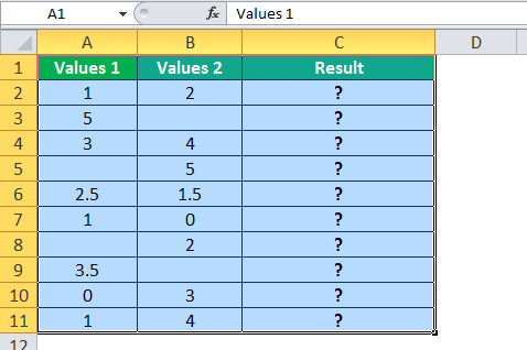
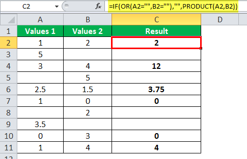
For example, B2 has an empty cell, so the result should be an empty value in cell C2.So, we will use the IF condition along with the OR function. If either of the cell values is nothing returned, nothing else returns the product of the numbers.

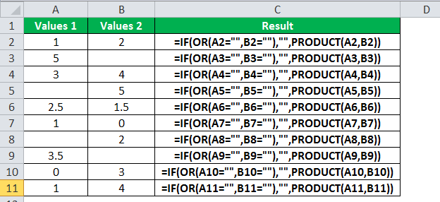
So, the PRODUCT formula in Excel that we will use is:

=IF(OR(A2="",B2=""),"",PRODUCT(A2,B2))

Applying the PRODUCT formula in Excel to each cell, we have:

Output:

Example #2 - Nesting of Product Function

When a PRODUCT in Excel is used inside another function as an argument, this is known as the nesting of a PRODUCT function in Excel. We can use other functions and can pass them as an argument. For example, suppose we have four sets of data in columns A, B, C, and D. We want the product of the sum value from the first and second datasets with the sum of values from the third and fourth datasets.

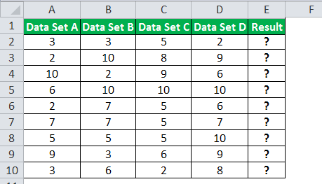
So, we will use the SUM function and pass it as an argument to the PRODUCT function in Excel. We want the product of the sum of the value of “Dataset A” and “Dataset B,” that is, 3+3 multiplied by the sum of the value of “Dataset C.” The“Dataset C,” value is (5+2), so the result will be (3+3)*(5+2).

=PRODUCT(SUM(A2:B2),SUM(C2:D2))

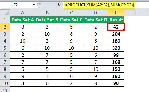
In the above example, the sum function is passed as an argument to the PRODUCT function in Excel. It is known as nesting. But, of course, we can do other functions also.

Example - #3

For example, suppose we have six divisions with a different number of persons employed for work. We have two tables with the numbers of persons in each division and the work hour of each person in each division. We want to calculate the total work hour of each division.

So, we will use the VLOOKUP function to lookup the values from both the tables and then pass it as an argument to get the total number by multiplying the number of people by the work hour per person.

So, the formula with Nested VLOOKUP will be,

=PRODUCT(VLOOKUP(G2,$A$2:$B$7,2,0),VLOOKUP(G2,$D$2:$E$7,2,0))