Power Query in Excel

Power Query is an excel tool used to import data from different sources, transform (change) it as required, and return a refined dataset in the workbook. Every change made to the data is recorded and saved as a step. In future, whenever the data source is updated, the same changes are performed automatically with the click of the “refresh” button.

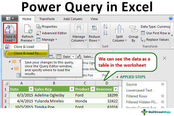
For example, an organization has 180 files containing the purchases made in the last 15 years. To consolidate and analyze these numbers, either of the following steps can be performed:

• Open the different files and copy-paste the entire data in one worksheet. Apply the various functions of Excel to convert the data into meaningful reports.
• Use Power Query to import data from the different files. Set up a query which consists of making step-by-step changes to the data. Load the transformed data in a worksheet to create reports.

If the organization follows the pointer “a,” it will have to perform a lot of manual work. These tasks are often tedious and repetitive. However, if pointer “b” is followed, the transformations are performed automatically every time data is updated. This saves a lot of time and speeds up the process of consolidating excel data.

Power Query in excel performs the extract, transform, and load operations (ETL) on a dataset. All transformations (steps or changes) applied to the data are collectively known as a query. By performing these transformations, the data is said to be shaped.

The major advantage of Power Query in excel is that it is a fast and efficient way of working on large datasets. Besides, it is reusable as the same query can be used again on a new dataset. Moreover, with just a few clicks, one can have access to cleansed and sorted data.

Power Query can be installed as an add-in in Excel 2010 and 2013. In Excel 2016 and the subsequent versions, Power Query is a built-in excel feature. It can be accessed from the “get data” drop-down (in the “get and transform data” group) of the Data tab of Excel.

To use Power Query in Excel, the following steps need to be performed:

1. Import data: Import data from the different sources. The data source can be a text file, Excel workbook, web, pdf, and so on. With Power Query, one can work with data from any source having any size and shape.
2. Transform data: Change, sort and shape data as per the requirements. For instance, one can delete or insert a row and/or column, replace a missing value, delete a duplicate entry, filter a column, and so on. These changes are recorded as a query in the sequence in which they are applied to the data.
3. Consolidate data: Consolidate or combine the data from the different sources. Once integrated, a consolidated database can be generated. The merging and appending of queries are carried out at this stage.
4. Load data: Load the data on a worksheet once it has been transformed and consolidated. Loading the data helps return an output in the workbook. The output can be in the form of a table, pivot chart or a pivot table. Prior to loading, one can preview the data to ensure it is on the right track.

Note: Each step performed (in pointer 2) is recorded and written in a code of M language.

The following image shows two Excel files (“data” and “salesdat”) and two text files (“year 2015 data” and “year 2016 data”). We want to perform the following tasks:

• Import all these files (Excel and text files) to the Power Query editor.
• Combine the data of the two text files. Extract this data as a single table and load it to an Excel worksheet.

The steps to perform the given tasks are listed as follows:

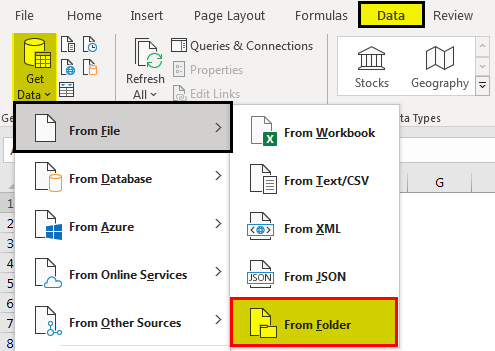
Step 1: To import data, click the drop-down of “get data” (in the “get and transform data” group) from the Data tab of Excel.

Open the options of “from file.” Select “from folder,” as shown in the following image.

Step 2: Click “browse” and look for the folder containing the text files (shown in the first image of this example). Select the correct path of the folder and click “Ok.”

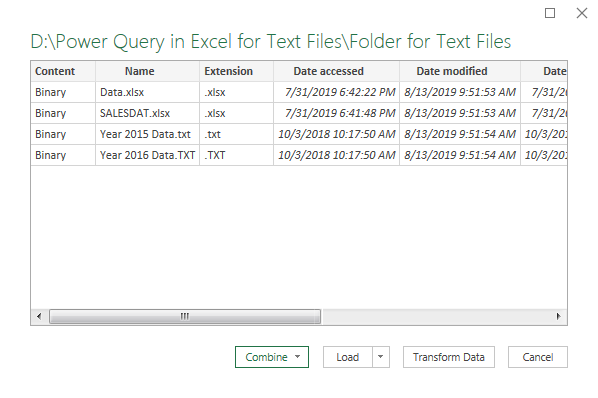
Step 3: A dialog box opens containing the list of files in the selected folder. The same is shown in the following image.

The column headers of this box are “content,” “name,” “extension,” “date accessed,” “date modified,” “date created,” “attributes,” and “folder path.”

At the bottom of this box, the following options are displayed:

1. Combine: This combines all the files of the folder. In other words, the user is not given an option to select the files to be combined. The combine drop-down shows the following options:
   • Combine and transform data–This helps consolidate all files with a query. Then, it opens the “power query editor” window.
   • Combine and load–This helps create a query and load the data to the worksheet.
   • Combine and load to–This opens the “import data” window after a query has been created.
2. Load: This displays the following options:
   • Load–This loads the data as tables in the worksheet.
   • Load to–This opens the “import data” window, which shows more loading options.
3. Transform data: This helps create a query and open the “power query editor.” Moreover, it allows choosing the files to be combined. So, one can combine the files having the same extension.

Since only the text files (with extension “.txt”) are to be combined, click “transform data.”

Note: Use “combine” when the folder contains only those files that are to be combined. Use “transform data” when the files to be combined are to be chosen after filtering.

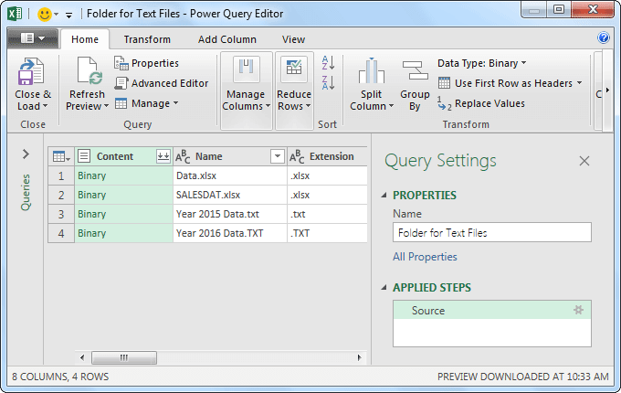
Step 4: The “power query editor” window opens, as shown in the following image. The Excel and text files have been imported to this window.

On the right side, the “query settings” pane is displayed, which consists of “properties” and “applied steps.” Connection with the source folder is the only applied step at present.

Further, there are three columns named “content,” “name,” and “extension” on the left side. The extensions are shown (in the column “extension”) in both lowercase and uppercase.

Step 5: Convert all the entries of the column “extension” to lowercase. This is being done because we need to filter the text extensions in the subsequent step (step 6).

For changing the case, select the column “extension” and click the “format” drop-down. Select “lowercase,” as shown in the following image.

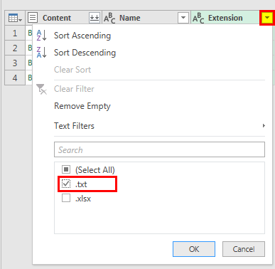
Step 6: Once all the entries of the column “extension” are displayed in lowercase, apply the filters. For this, click the drop-down arrow of the column “extension.” The options of this menu are displayed in the following image.

Since the data of only the text files are to be extracted, select the checkbox of “.txt” and click “Ok.”

Step 7: To combine the data of the two text files, click the icon displaying near the header “content.” The same is shown within a red box in the following image.

Note: Prior to combining files, ensure that they all have the same extension and structure.

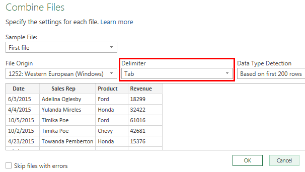
Step 8: A dialog box captioned “combine files” opens, as shown in the following image. Select “tab” as the “delimiter.” This is because a tab separates the entries of the text files.

In “data type detection,” select “based on first 200 rows.” This implies that the data type detection needs to be done on the first 200 rows of the dataset.

One can preview the data of the combined text files on the left side of the “combine files” window. If the preview is fine, click “Ok.”

Note: By default, the first file of the list is used as the sample file. However, one can select a different file as the sample file. For this, use the drop-down menu under “sample file”.

Step 9: The “power query editor” window opens. It shows the data of the combined text files as a single table.

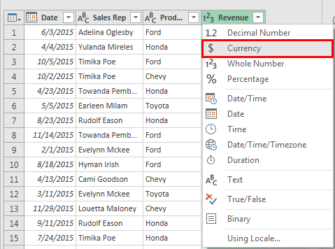
Step 10: Add transformations to the extracted dataset. Change the data type of the “revenue” column to “currency.” For this, click the drop-down near the header “revenue” and select “currency.”

The same is shown in the following image.

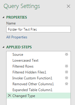
Step 11: The number of applied steps has increased, as shown in the following image.

Note: One can click on any of the “applied steps” to see how data appeared after applying the specific step.

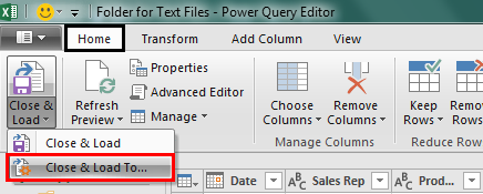
Step 12: Once the transformations to the data are complete, load the combined dataset to an Excel worksheet. For this, click the drop-down of “close and load” (in the “close” group) from the Home tab of the “power query editor” window.

Select “close and load to,” as shown in the following image.

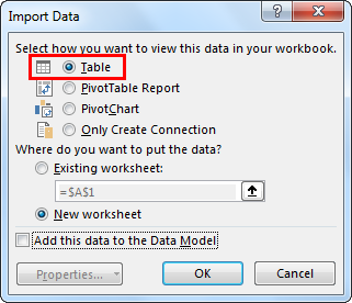
Step 13: The “import data” window opens, as shown in the following image. Select the kind of output required in the worksheet.

Since we want the output in the form of a table, select “table” and click “Ok.”

Note: One can create just a connection with the data by selecting the option “only create connection.” When a connection is created, no output is returned in the workbook. However, the query and the steps applied are saved. This query can be used in other queries.

Step 14: The combined data of the two text files (shown in the first image of this example) appears as a table on the worksheet. Hence, the text files of the D drive have been imported, consolidated, transformed, and loaded in Excel.

Step 15: One can view the list of workbook queries under the “queries and connections” pane. This pane can be used for navigating, editing, merging, duplicating, appending, and deleting queries.

The following image shows that 601,612 rows have been loaded by Power Query in excel. Hence, by using Power Query, a transformed output has been obtained within a short span of time.

Note 1: One can revise (modify) an existing query with the help of the “edit” option. By revising a query, the steps applied to the data can be edited, deleted or reordered.

Note 2: One can refresh a query when new data is imported. As a query is refreshed, the associated charts, tables, and other data forms are automatically updated.

The important points related to the usage of Power Query are listed as follows:

• Excel Power Query does not make any changes to the original (source) data file. It simply records the transformations made to the dataset. Then, it returns the refined dataset in the workbook.
• Power Query is case-sensitive. This implies that it distinguishes between the lowercase and uppercase versions of the same text.
• Power Query imports temporary files as well. So, such files must be excluded before the consolidation of data. One can filter the “extension” column to exclude the temporary files.

Note: The names of the temporary files begin with the tilde symbol (~). They have the “.tmp” or “.temp” extension.

This has been a guide to Power Query in Excel. Here we learn how to use Power Query to manage our data in Excel with the help of step-by-step examples. You can learn more about Excel from the following articles-

• Power BI Query Editor
• Power View in Excel
• Data Model in Excel