Pivot Table From Multiple Sheets

Publication Date :

19 Mar, 2019

Blog Author :

Edited by :

Reviewed by :

Download FREE Pivot Table From Multiple Sheets Excel Template and Follow Along!

Pivot Table from Multiple Sheets Excel Template.xlsx

Table Of Contents

Excel Pivot Table From Multiple Sheets

PivotTables from multiple sheets are a concept where we should add two or more tables to one table. Then, we can select the fields according to the requirement from one place.

In a word, it means different tables. Data can be appended from other sheets using some techniques and shortcuts.

How to Create a Pivot Table from Multiple Sheets?

Implementing PivotTables from multiple worksheets has some different processes. This process can also be done in different ways. The following are the other methods to create a PivotTable from multiple sheets in Excel.

Process #1

The no. of sheets should be two or more.

For this process, we need data on multiple worksheets. E.g., Sheet1, Sheet2, Sheet3, etc.

Below are the steps to create a PivotTable from multiple sheets:

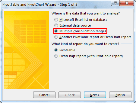
First, click "Alt+D," then click "P." The following dialog box will appear.
Select "Multiple consolidation ranges" in that dialog box and click "Next."
After clicking "Next," it will go to Step2. In that, select "I will create the page fields" as in the below dialog box.
After selecting the above options, click on "Next" again. The window also will be moved to the third step. In this step, it will open another step after clicking the "Next" button as shown below.
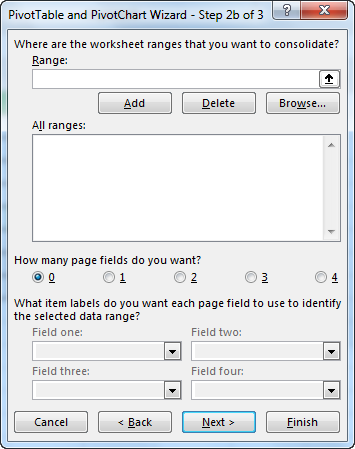
In that, select the range of table 1, click the "Add" button, and select the range of another table in another sheet. Then, click "Add." Now, it will add the two tables to a single table.
Select the page field as "1" below the "All ranges" option. Then give the names to the two sheets as per the better understanding so that if we click table 1, it will show the table name in the PivotTable for better knowledge.
There is an option to select whether we will insert the PivotTable in a new or existing worksheet. A new worksheet will be selected, as shown in the figure.
Finally, click on "Finish." Now, it will create the PivotTable in a new worksheet.
By default, it will show the "Count of Value." We should change the value in the headings for the sum. For that, go to any cell which contains a value and right-click. Then, select the "Summarize Values" option.
After this, we can remove the columns we need and do not need. We can do this by selecting the “Column Labels." Then, we can check the column labels, whichever is necessary.
Now, there is the other column for grand totals. In general, we do not need the grand totals of columns. Hence, that can be removed by right-clicking on the value and selecting "PivotTable Options." A dialog box will appear, as shown below.
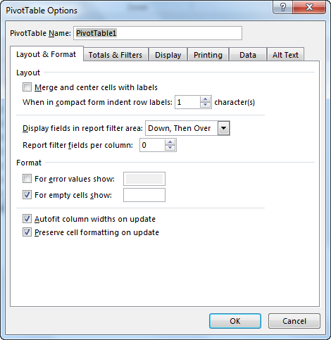
Go to the “Totals & Filters” tab and uncheck the option "Show grand totals for rows." If necessary, we can retain it or uncheck the option for it. Now, click on "OK."
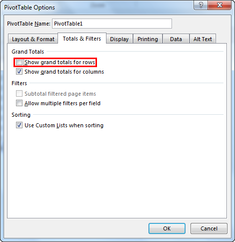
Now, the grand totals will only be present for the columns.
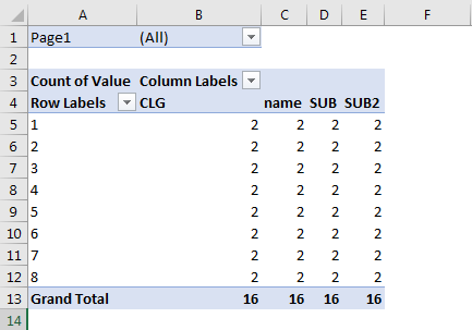
The final step would be changing the name of the PivotTable. Again, it can be user-defined or related to the data in the PivotTable.

It is the first process to create a PivotTable from multiple sheets in Excel. In this PivotTable, as in the normal PivotTable, only the fields from the right side can be dragged and dropped as per the requirement.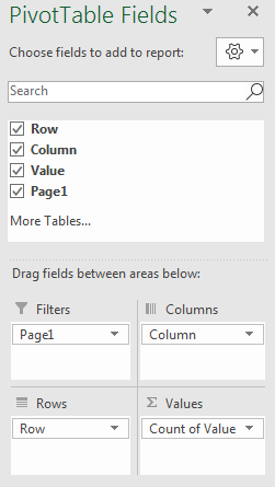

Process #2

In this method, there should be a common row in both tables. It will act as the primary key for the first table and the foreign key for the second table.

Here, we will use Sheet 4 and Sheet 5 to create a PivotTable from multiple sheets in Excel.

We will analyze the second method with the help of the following example.

Step 1: In sheets 3 and 4, select the table, click "CTRL + T" to select the whole data, and draw a table for complete data. Now, it will insert a table in the data. The name will be displayed on the table in the left corner. This process can be done for all the tables containing the data.

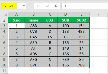
It will add filters in default. If we do not need them, we can turn them off by clicking the "CTRL+SHIFT+L" shortcut from a keyboard or going to the “Data“ tab and clicking on the "Filters" option. Then the filters will be disabled.

These are the steps to be followed to create a PivotTable for the following data.

Step 1: Click on the "Insert" tab and "PivotTable." A dialog box will appear now, and you will be asked whether we should create the PivotTable in a new or the same sheet.

It is good to use a new sheet option in excel.

Step 2: Lastly, check the box “Add this data to the Data Model.” It is an important step in this PivotTable creation process.

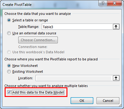
Step 3: A PivotTable will be created now in the new worksheet. On the right side, we may have all the fields related to the PivotTable.

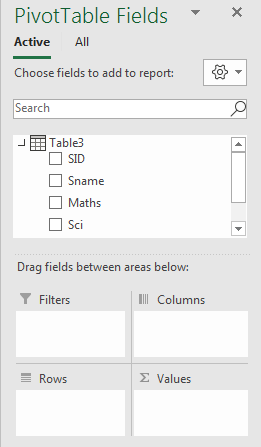
Step 4: Go to the “Analyze” tab -> Relationships -> New.

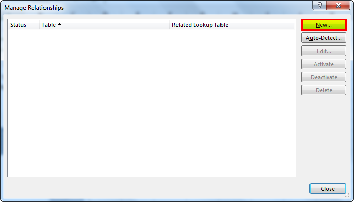
Step 5: The table is the current table. The related table is the table to be added to the PivotTable. The corresponding column is the same in both tables. It is from the first table, also called the primary key. A column is the same in the second column, called a foreign key.

Step 6: Now, click on the ok.

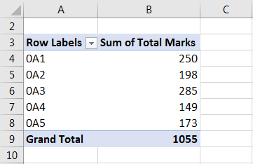
Step 7: Now, we can select the required fields per the requirement. We can choose the fields from all the tables in the PivotTables. For that, it will first ask to create a new PivotTable.

Step 8: Click "Yes." We can select fields from all the tables to create a PivotTable.

Process #3

The first and foremost thing in this method is to assign a name to all the data. We will illustrate this by an example. Below is an example of this process.

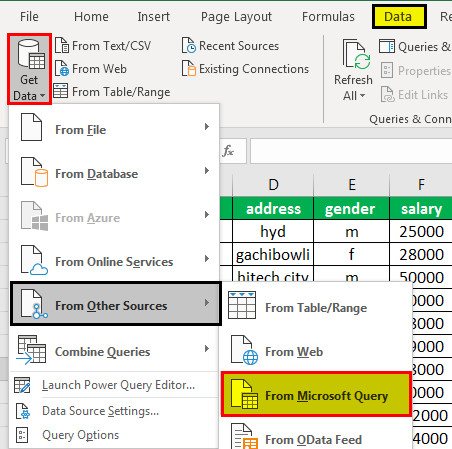
Step 1: Create a table for the entire data by pressing the"CTRL+T" shortcut keys and removing filters. Now, Go to the “Data” tab -> click on “From Other Sources “ -> From "Microsoft Query "-> Excel Files.

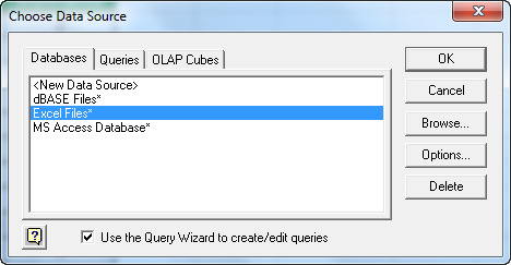
Step 2: Select the worksheet in which you have created the data.

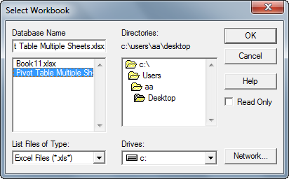
Step 3: This step will show another window to select the tables of all the sheets in the workbook. The tables can be chosen as per the requirement, as shown below. We have chosen sheets 5 and 6.

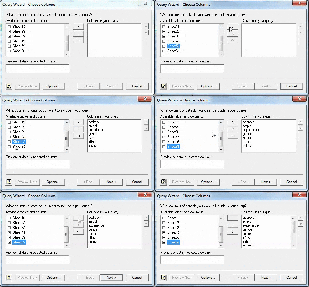
Step 4: After selecting the tables from the sheets, click "Next." You will get this dialog box and click on "OK."

This dialog box says that without joining the tables, the query cannot be executed and now join the tables.

Step 5: Then, a window will appear. In that, all the data belonging to all the tables will be present. There will be two portions in that window: “ Name Range, “and " Data Area."

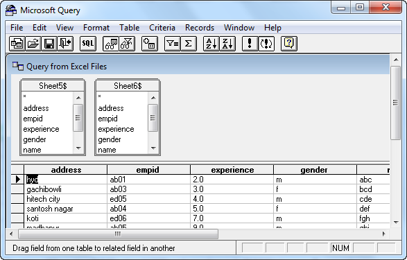
Step 6: Go to the "File" menu and select “Return Data to Microsoft Excel.”

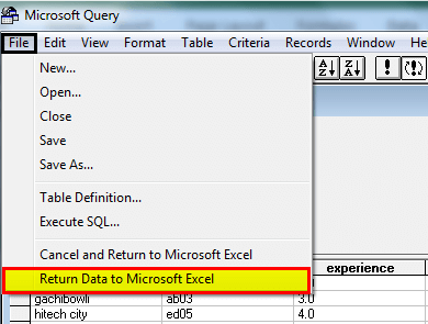
Step 7: Now, you will get a window of “Import Data."

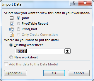
Step 8: In this window, as we want to create a PivotTable, select the option “ PivotTable Report “ and click on "OK."

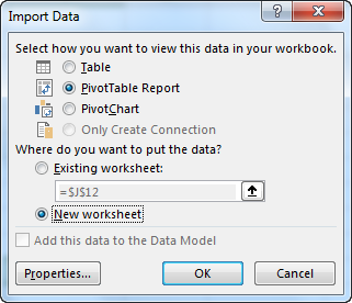
Step 9: The PivotTable is ready. We can create it as per the requirement.

Note: The reason for inserting a table into the data is that if, in the future, any data is appended in the last, then the Pivot Table can be refreshed by new data automatically by just refreshing the page.

Things to Remember

There should be two or more tables in one workbook for creating a PivotTable.
If any new data is added to any of the tables after creating a PivotTable, then to reflect the changes, we need to refresh the PivotTable manually.
Every time we create a PivotTable, we should make it in a new worksheet to reflect the changes correctly.
When we drag and drop in excel, the attributes from any of the tables into four fields, it will generate the report's summary in just a few seconds.
The main thing in creating a PivotTable is that no cell, column, or row should be left blank if there is no value. It should be “0” or any other value. Else, the PivotTable will not be shown up correctly.
Quick Tool Tip: The PivotTable quick reference can be added to the quick toolbar using the following process.

Click "Customize Quick Access Tool Bar", go to "More Commands" -> Popular Commands -> Select PivotTables -> click on "ADD."

It will add the PivotTable option to the quick access toolbar for easy access.