Pivot Table Examples

PivotTable is a table of stats that summarizes the data as sums, averages, and many other statistical measures. Let us assume that we got data of any real estate project with different fields like type of flats, block names, area of the individual apartments, and their other cost per various services, etc.

• Pivot Table sums up data through statistical measures like sums and averages. 
• It eases the analysis of large amounts of data, such as in real estate projects with various flat types, block names, individual apartment areas, and service costs.
• To select a row or column, tap its letter or number.
• In Excel, modifying the format creates a duplicate format. Custom number formats affect the cells' appearance, not their values. On custom format removal, cells are present in the default format.

Below is the raw data for the PivotTable practice exercises.

Create a PivotTable using the above table.

PivotTable Example #1 - Performing Statistics Measures In PivotTable

SUM:

In the Excel Pivot Table Example, we should perform the sum of the final product value to extract the value of different blocks got as below:

Drag the "Block Name" to "Rows" and "Sum of Final Product Value" to "Values" Fields.

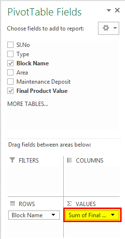
It shows that we have the "Cheeku" block with 293 million, "Donald" block with 212 million, "Mickey" block with 324 million, "Rainbow" block with 466 million, and "Strawberry" with 355 million. This table shows us that the "Rainbow" block got a higher value than the other blocks.

COUNT:

Let us count the number of flats for different blocks by changing the value field settings in Excel PivotTable to count as below:

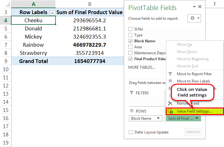
Then, click on "Value Field Settings."

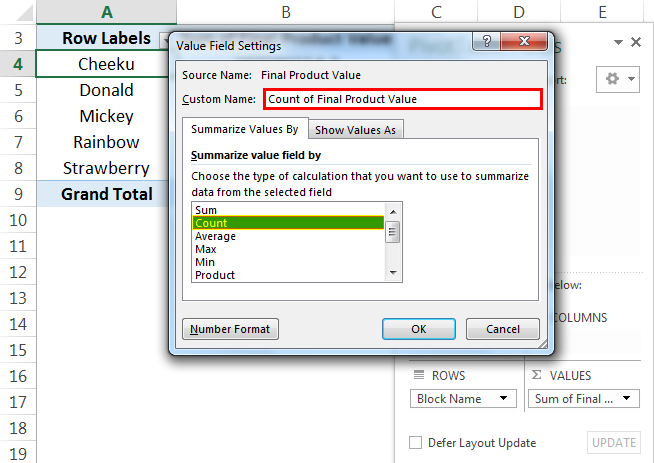
A dialog box appears. Select “Count” from "Summarize value field by."

Then the PivotTable looks like as given below:

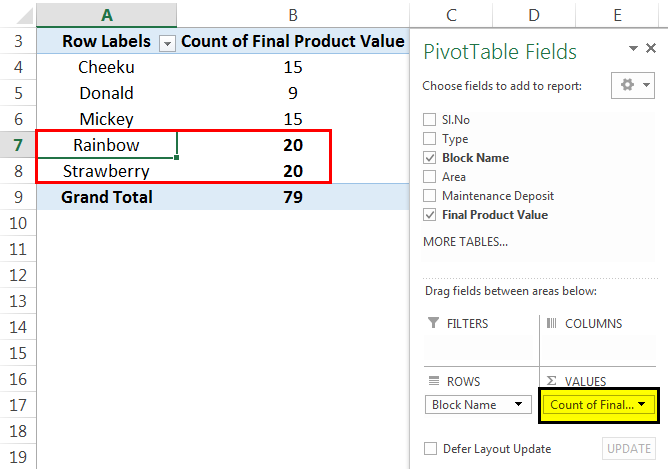
From the above tables, we can see how to change the field settings to count. Here, we can note that we got the highest number of flats in the "Rainbow" block and "Strawberry" block compared to other blocks. In total, we got 79 flats in this project.

AVERAGE: 

In the PivotTable practice exercise example, we will find out the average price of the flat in each block by changing the value field settings from "Count" to "Average."

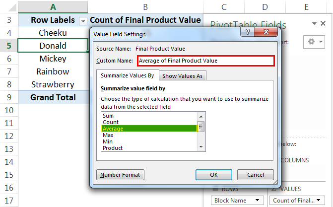
Then, PivotTable changes from "Count" to "Average," as given below:

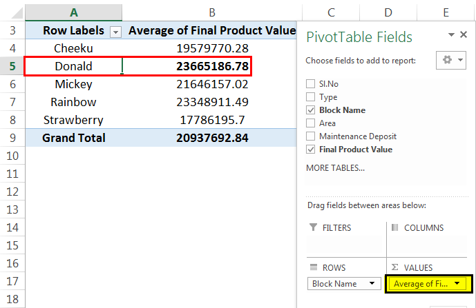
From the above PivotTable example, we can see that we got the average flat price in each block. The "Donald" block got the highest average flat price among other blocks.

Similarly, we can perform other statistical measures like Max, Min, Product, Standard deviation, etc., by changing the value field settings in this PivotTable example.

Pivot Table Example #2 - How Can We Modify The PivotTables In Excel

We can change the layout of the Excel PivotTable per our requirement by dragging the fields into areas where we want to place them.

In this example of a PivotTable in Excel, let us see how it works.

First, we must drag the “Maintenance Deposit” into the "Values" area to check each block's total maintenance price. You will get your table modified as below:

This PivotTable shows both maintenance deposit and an average price for different blocks. As discussed earlier, we can change the statistical measure by changing the value field setting.

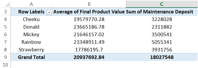
We can also modify the above table further by adding the type of units that are available as block-wise as below:

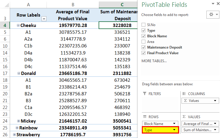
The above table shows that the type of flats in the "Cheeku" block are A1, A2a, B1, B2a, C1a, C1b, D1c, D2b, D3b, D4a, D4b, D4c. Similarly, we get for other blocks too.

Pivot Table Example #3 - Grouping The Fields In The Excel PivotTable

We can also create a group in Excel PivotTables to differentiate a few fields. In our PivotTable practice exercise example, let us create the "Strawberry" block, "Cheeku" block as "Group-1" and "Donald" block, "Mickey" block, and "Rainbow" block as "Group-2."Let us see how we can create these groups:

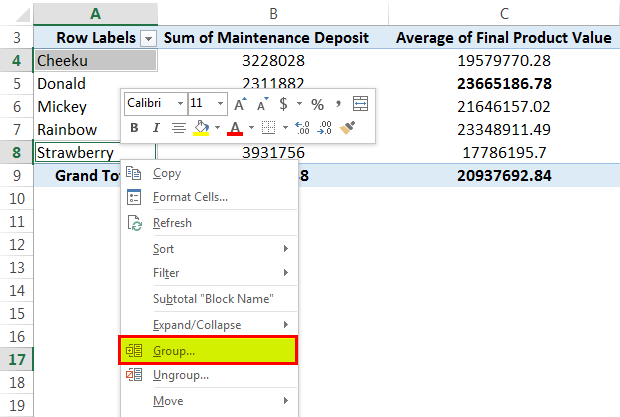
As per our above PivotTable example, select "Cheeku" and "Strawberry" with the help of the "Ctrl" key. Then, right-click on the mouse to get the list. Next, go to the "Group" option and then click on it.

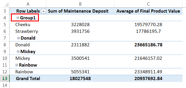
Now, we can see the group has been created as below:

Similarly, we can select the rest of the block and do the same. Then, click on the "Group" again. Now, "Group-2" will also be created as follows:

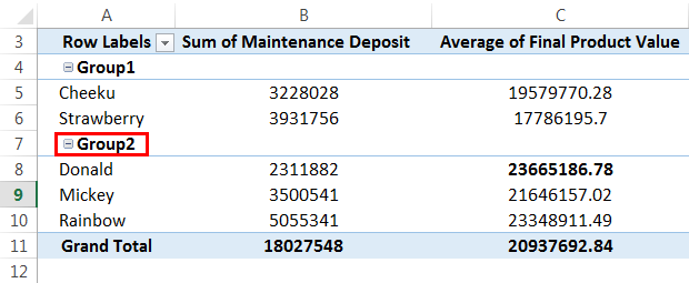
We can also name the group by editing the group and giving the names per our requirements.

PivotTable Example #4 - Creating Multi-Levels In Excel Pivot Table

Creating multi-levels in PivotTable is easy by just dragging the fields to any specific area in a PivotTable.

But here, in the example of the PivotTable, we understand how we can also make great insight into this multilevel PivotTable.

First, we need to drag the "Block Name" into "ROWS" as we find some insight into the block of the project. Then, drag the "Final Product Value" to the "VALUES" area as we get the sum of all flats units value of a particular block in the table.

Drag the "Final Product Value" to the "VALUES" area to create a multi-level table.

We can see the table with two columns with "Final Product Value" for different blocks below:

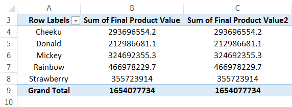
Now, let us find out some insight from this data. To do so, we should change the value field set to any measures that need to be considered. Here, we will take a percentage to see the contribution of different blocks in terms of the product value as below:

Go to "Value Field Settings," then select “Show values as.” In that, select “% of Column Total.”

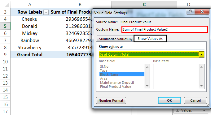
We can see the table with a percentage in "Sum of Final Product Value2" below:

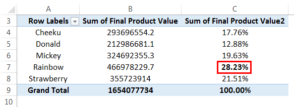
From the above data, we can understand that the "Cheeku" block had contributed 17.76%, "Donald" – 12.88%, "Micky" – 19.63%, and "Rainbow" – 28.23%, and "Strawberry" – 21.51% of the total value of the project. A "Rainbow" block is the highest contributor among all other blocks.

Similarly, we can perform different multi-level operations using a PivotTable, which provides great insight into the data.

PivotTable Example #5 - Creating Frequency In Excel PivotTable

Earlier in the example of the PivotTable, we had seen grouping the name of the blocks. Now, let us group the value to create a frequency that shows us the number of units that fall under a certain area category.

First, drag the area field into "ROWS" and again drag the same area field into the "VALUES" area. By default, the "VALUES" area gives the sum of the area, so we should change it to count because here, our goal is to find several units in a particular area category.

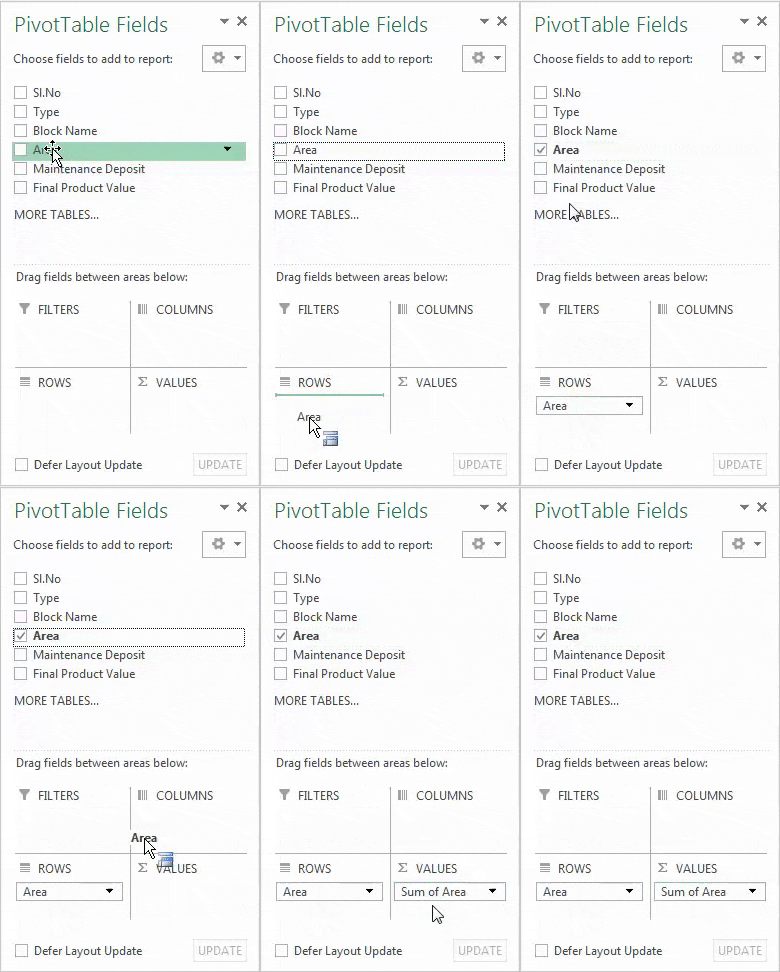
Now, right-click on any cell of the row labels and the select group.

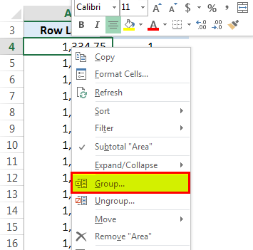
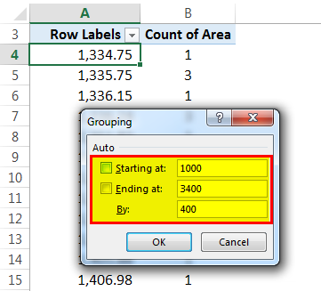
Then, the "Grouping" window will pop out where we have to give the starting number for the frequency to get started and the ending number. In addition, we have to provide a number that will create a frequency.

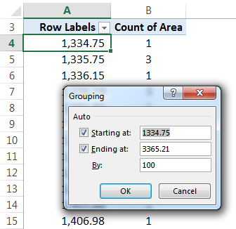
Let us provide the conditions as a starting point as 1000 and ending at 3400. Then, it should be split by 400.

Now, we can see that the area category has been formed. There are 19 flats which got an area between 1,000-1,400 sq.ft, 5 flats with an area between 1,400-1,800 sq.ft., 41 flats with an area between 2,200-2,600 sq.ft., 2 flats with an area between 2,600-3,000 sq.ft. and 12 flats with an area between 3,000-3,400 sq.ft. So, here we can assume that we got the highest number of flats with 3 BHK configurations per area.

You can download this Pivot Table Examples Excel Template here - Pivot Table Examples Excel Template

• Pivot Table helps us analyse large dataset used in various fields such as gaming, finance, auditing, business projects etc.
• We can use statistical functions to create accurate Pivot Tables useful for the users.
• To select the entire sheet, remember that we need to click on the box next to "A" or above "1."

This article is a guide to PivotTable examples in Excel. Here, we provide practice exercises PivotTable in Excel with examples such as modifying PivotTable, statistical measures, and grouping fields. You may learn more about Excel from the following articles: -

• Excel Pivot Table Count Unique
• Create a Pivot Table From Multiple Sheets
• Use the Pivot Chart in Excel
• How to use a Pivot Table Filter?