Pivot Table Calculated Field & Formula

Publication Date :

03 Jul, 2023

Blog Author :

Edited by :

Reviewed by :

Download FREE Pivot Table Calculated Field Excel template and Follow Along!

Pivot Table Calculated Field Excel template.xlsx

Table Of Contents

What Is Pivot Table Calculated Field & Formula?

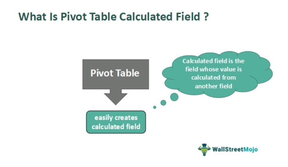
Pivot Table Calculated Field & Formula refers to the Pivot Table feature that simplifies creating calculated fields. A calculated field is one that derives its value w.r.t other fields. It helps in making the analysis of data easy and smooth, thereby facilitating smoother decision-making.

For example, we can visualize this feature as shown in the image below.

Pivot Table Calculated Field & Formula — *You are free to use this image on your website, templates, etc..* *Please provide us with an attribution link.*

The Pivot Table calculated field allows the data to be organized in a sequence and be used for calculating the fields that are dependent on the values contained in the other fields. The feature enables users to feed the data without hassle.

Key Takeaways

The Pivot Table Calculated Field & Formula helps users comprehend the generated PivotTable in relation with the other calculated fields and formulas.
We can create PivotTable Slicers too, to breakdown the Pivot Table into more simple tables.
When we generate a PivotTable for a dataset, we can modify the data within the selected cell range for the PivotTable to get updated.
However, if we add more rows and columns, it will not reflect on the generated PivotTable.
In such scenarios, we can make the PivotTable into a Dynamic Table to overcome the issue.
We can also use the Conditional Formatting to highlight the desired data in the Pivot table that is generated.

Pivot Table Calculated Field & Formula Explained

Pivot Table calculated field & formula arranges values in different fields in a proper sequence and allows users to handle the data either through manual reference or by using the formula.
The calculated fields derive their value from the other fields fed in the data set. This organized set of data makes it easier for analysts to analyze the details and make well-informed, wise decisions.
We can use some basic mathematical operations inside the calculated fields in the Pivot Table. However, we cannot use the logical and other thread functions.
A Cell reference will not change if the reference is generated via the GETPIVOTDATA function.
The calculated field formulas are also a part of a PivotTable. If there is a change in the source data, then the formulas will be unchanged until the pivot table is refreshed,

How To Add/Edit The Pivot Table Calculated Field & Formula?

To Add/Edit the Pivot Table Calculated Field & Formula, we must,

First, select the data range, and generate a PivotTable.
Next, click the generated Pivot Table to get the Analyze and the Design Tabs on the ribbon.
Finally, click the “Analyze” and the options to “Insert the Calculated field”.

Let us understand the same with an example.

The steps to Add/Edit the Pivot Table Calculated Field & Formula are as follows:

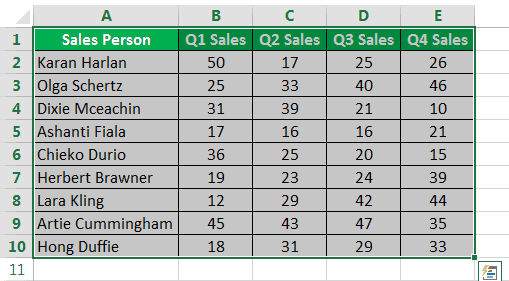
Select the data that is used to generate the PivotTable.
Go to the ribbon and select the “Insert” tab. From the “Insert” tab, choose to insert a “PivotTable.”
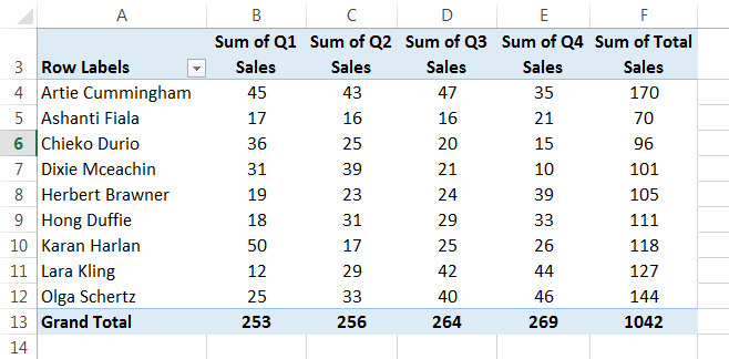
Select the “PivotTable Fields” such as “Sales Person” to the “ROWS” and Q1, Q2, Q3, and Q4 sales to the “Values.”

Now, the PivotTable is ready.
After the PivotTable is inserted, go to the “Analyze” tab, that will only be present if the PivotTable is selected.
From the “PivotTable Analyze” tab, choose the option of “Fields, Items Sets” and select the “Calculated Field” of the PivotTable.
In the option of “Insert Calculated Field” in the Pivot Table, insert the formula as required in the case.

Here, we have formulated a formula to calculate the 0.05% commission on sales.

How To Switching Off The “GetPivot” Table Function?

We can always switch off the “Getpivotdata” function using the “Analyze” tab. Here, go to the “PivotTable” group, as shown below.

Click the “Options” option drop-down, and click the checked “Generate GetPivotData” option to turn it off, as shown below.

Now, we can use the formulas in the PivotTable as we do in the case of a simple range.

Important Things To Note

Ensure to generate a PivotTable with a real-time existing dataset, because it will not work for blank rows or columns.
Anytime during the calculation, we can modify the calculated fields to get a new value.
Always remember to apply conditional formatting to the generated PivotTable and not to the dataset, when working with Pivot Table Calculated Field & Formula.