Percentage Change Formula in Excel

We can do arithmetic calculations via Excel formulas. One such calculation is “percent change” from one value to another. For example, suppose you want to find the percentage change between your first drawn salary and your current salary. In that case, that will be calculated in terms of the percentage change. It is possible in formulas in Excel. This article will discuss calculating the percentage change formula in excel.

A percentage change or percentage variance is the change between two values over time. For example, a specific percentage change is the “variance between last year's sales and this year's sales.”

For example, last year’s sale was $400,000. This year, sales are $450,000, so the difference is a $50,000 increase in revenue. But we can also tell this percentacge-wise.

So, to calculate the percentage change between two numbers is below.

Else, we can also use the below formula.

In the above example, the previous year's sales were $ 400,000, and current-year sales were $450,000. So, let us apply these numbers to the formula.

(Current Value – Previous Value) / Previous Value

= (450000 – 400000) / 400000

= 50000/400000

= 12.5 % increase in Revenue.

Now, we will see how we can apply the same formula in Excel.

Example #1

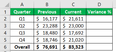
Below is the quarterly sales data for the previous and current years of ABC Co. Pvt Ltd.

From this data, we need to determine the variance percentage from the previous quarter to this year’s quarter.

Let us use our formula, as we have learned above. However, we will use cell references instead of entering the numbers directly into the formula.

Copy the above table to an Excel sheet.

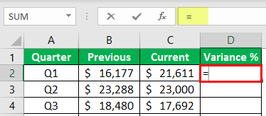
Now, put an equal sign in cell D2 because all the formulas in Excel must start with an equal sign only.

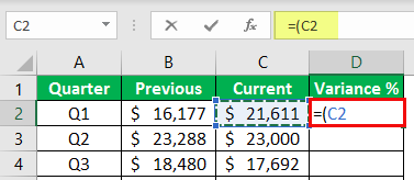
Open the bracket, and our first formula should be the current value. In this example, the current value is the C2 cell value.

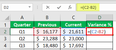
Then, put the minus (-) sign and choose the previous year's value,B2 cell.

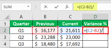
Close the bracket and put it divided by a symbol by inserting a forward slash.

Now again, select the previous year's value.

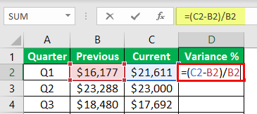
Press the "Enter" key to get the result of the percentage change from the previous year to this year.

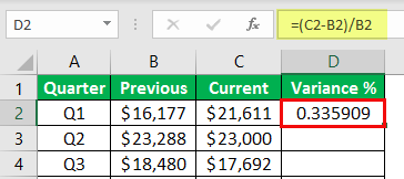
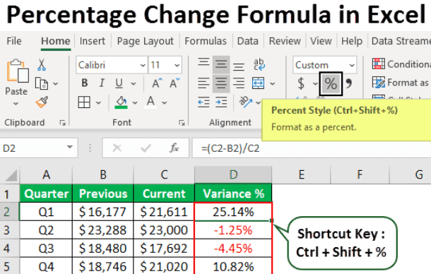
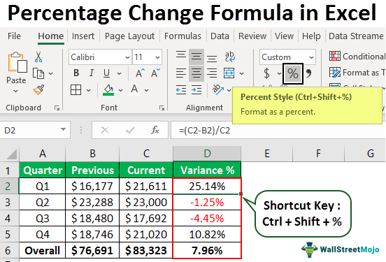
We got only decimal values. For this, we must apply the percentage format. To use the percentage format, select the cell, and press the percentage (%) symbol.

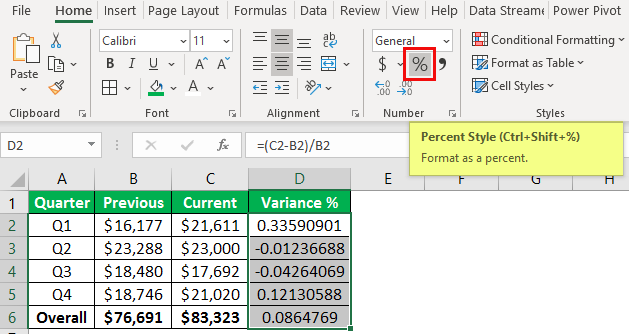
We can also press Ctrl + Shift + % as a shortcut key to apply percentage change. We can see the percent change values as soon as we use the percentage format.

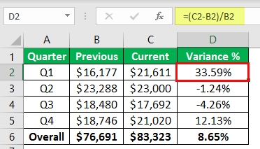
First, the percent change is 33.59%, the current revenue is 21611, and the previous revenue is $16,177. So revenue has increased from previous to this current year. So it increased by 33.59%.

Similarly, the second value percent change is -1.25% and revenue decreases.

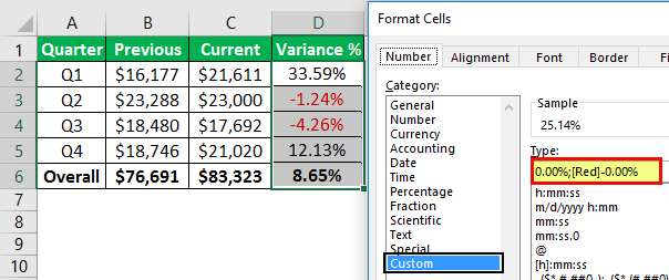
Use the formatting code below to apply the red color format to a negative percent change.

0.00%;-0.00%

Example #2

Below are employees' salary details and their current salary when they joined.

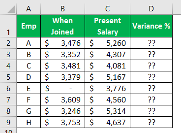
Let us use the same formula above to find the variance percent change between these two numbers.

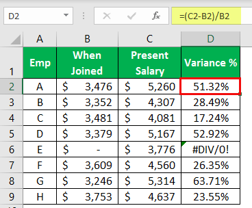
As we can see in cell D6, we got the error value because whenever we divide the number by zero, we get the division error value as #DIV/0!.

So to get rid of this, we need to use the IFERROR function in excel.

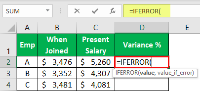
The first argument of this function is value. So for this, apply the percent change formula as usual.

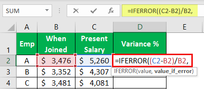
The second argument is value if error.It says what should be the value if the supplied calculation returns as the error value, so we need the result to be 0%.

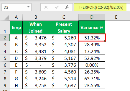
Now see, we got rid of the error value because of the IFERROR function.

Example #3

Below is the sales employee’s revenue generation comparison from last month to this month.

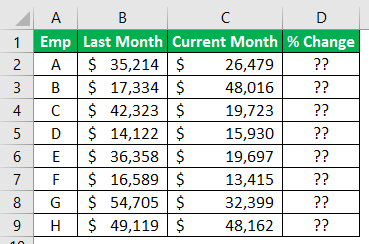
Below is the sales employee’s revenue generation comparison from last month to this month.

Current Value / Previous Value – 1

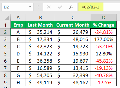
So, only two employees performed better than the previous month, D3 and D5 cells.

• We must always use cell references to make the formula dynamic.
• When dividing the value by zero, we may get a division error of #DIV/0!.
• We must use the IFERROR function to get rid of error values.