Table Of Contents
What Is Page Break In Excel?
Page Break in Excel is used to separate an Excel worksheet into multiple or different pages where the user can decide the format of the Page Breaks. The Excel Page Break is mainly used while taking printouts of the worksheet, to get the required data and not the entire worksheet.
For example, when we apply the Page Break feature on a dataset, we get the output shown below.
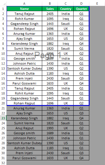
Table of contents
- The Page Break in Excel is a feature used to separate data in an Excel worksheet for printing purposes, and it can be inserted vertically and horizontally on a column or a row, respectively.
- We can insert, remove, move, hide, show, or reset the Excel Page Break.
- By default, during printing, the system decides how much content goes on one page. However, with the help of Page Break, we can separate the data as per our requirement and avoid misalignment.
- When we apply Page Break, we’ll still see the whole data in the worksheet. But in the Preview, we will see the Page Break, represented by a blue highlighted outline.
How To Insert A Page Break In Excel?
We can insert A Page Break, vertically or horizontally, as follows:
- First, select the cell where we want to apply the Page Break, here, cell C4.
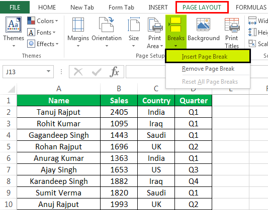
- Next, select the “Page Layout” tab → go to the “Page Setup” group → click the “Breaks” option drop-down → select the “Insert Page Break” option, as shown below.
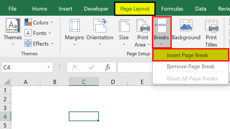
We can see the light grey lines that indicate the Page Breaks.

- Finally, to view the Page Break when we apply in a dataset, we must select the “View” tab → go to the “Workbook Views” group → click the “Page Break Preview” option.
Examples
We will consider some examples by applying the Excel Page Break.
Example #1 - Create a Vertical Page Break in Excel
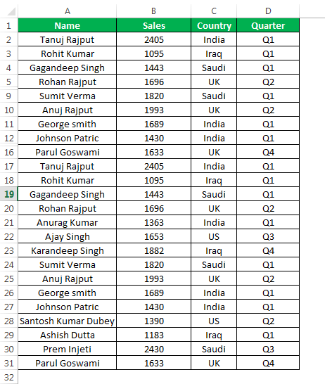
Let us consider the below dataset, to apply the Page Break to break the page vertically.
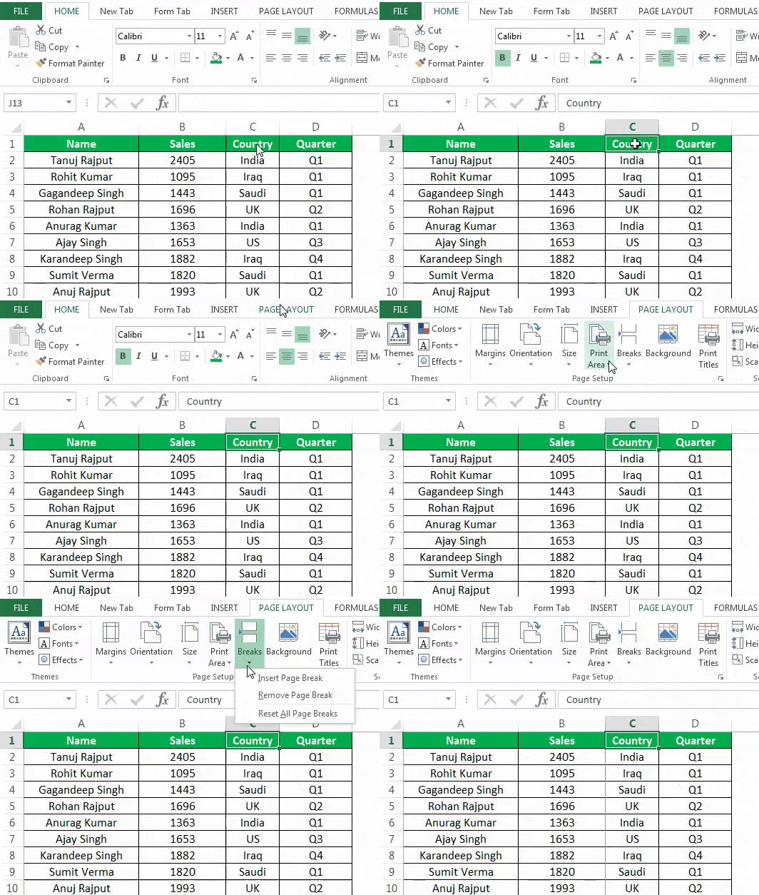
We must select any cell from row 1 where we want to place the Page Break. Here, we have chosen the C1 cell. But, first, go to the “Page Layout” menu, and select the “Insert Page Break” option.
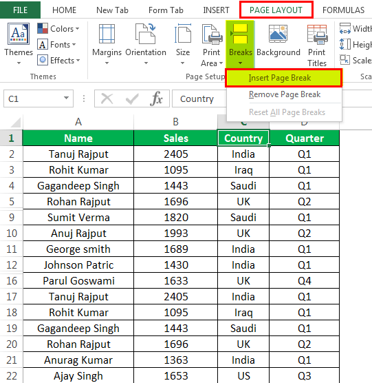
We can see a vertical line on your worksheet, as shown in the figure below, which indicates the Page Break we created.
Example #2 - Create a Horizontal Page Break
Let us consider the same sales data to apply the Page Break, but this time horizontally.
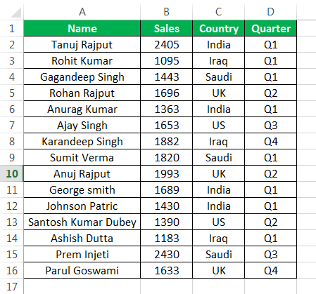
Select any cell in column A or right below the row where we want to insert the Page Break.
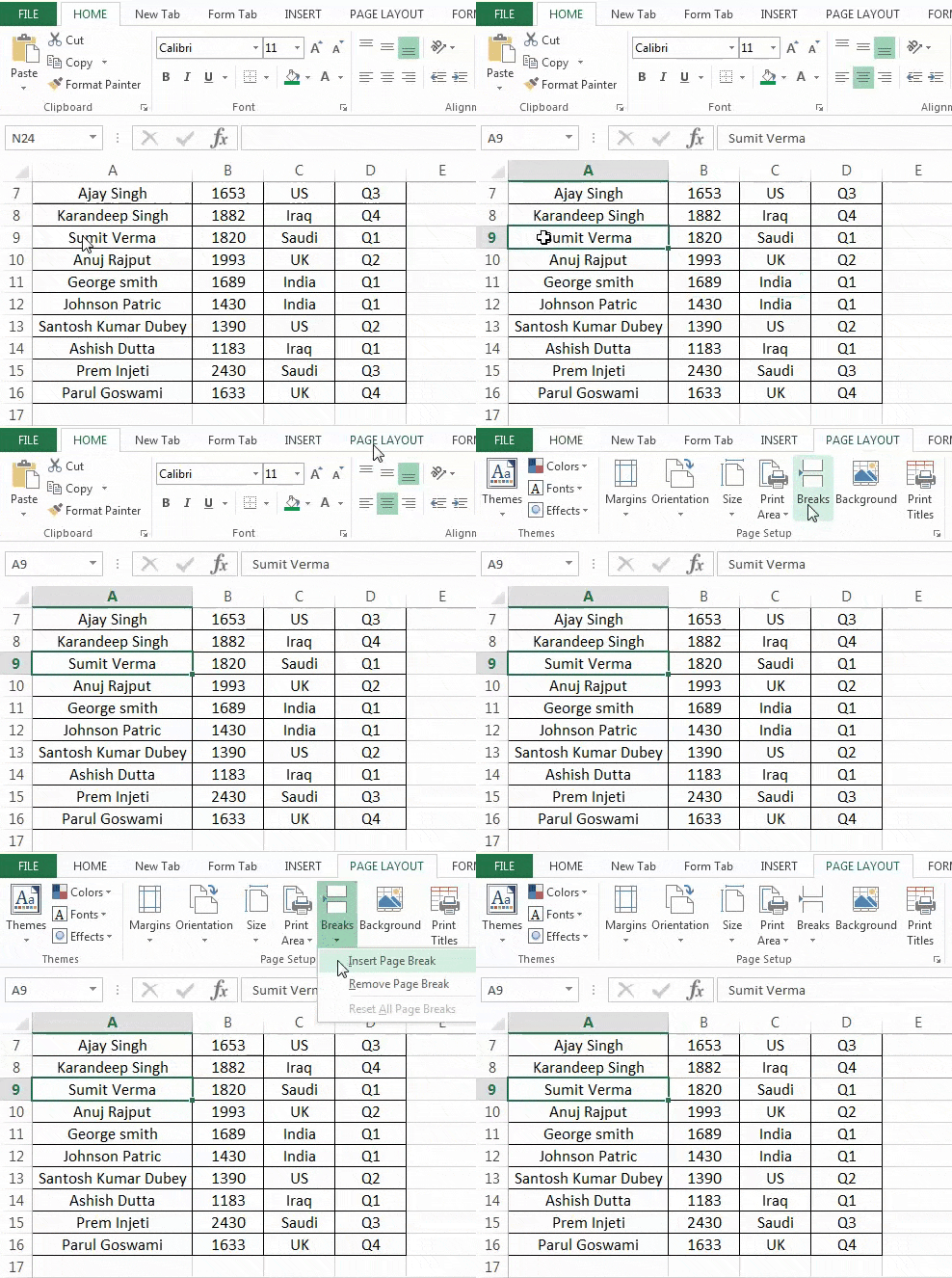
We selected the A9 cell, and applied the Page Breaks in this example. Next, go to the “Page Layout” menu, and select “Insert Page Break”.
The horizontal Page Break is inserted in the selected sales table. So, for example, we can check the horizontal Page Break in the below figure:
Example #3 - Move a Page Break
We can move the Page Break by using the below steps:
- First, we must open the worksheet where we need to modify or move the Page Break. Next, click on “View” and “Page Break Preview”.
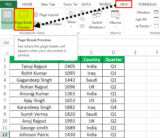
The “Page Break Preview” is shown below:

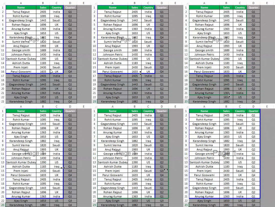
- We can move it from the simple dragging options shown below.
Example #4 - Delete a Page Break
The steps to delete or remove the Page Break from the worksheet are as follows:
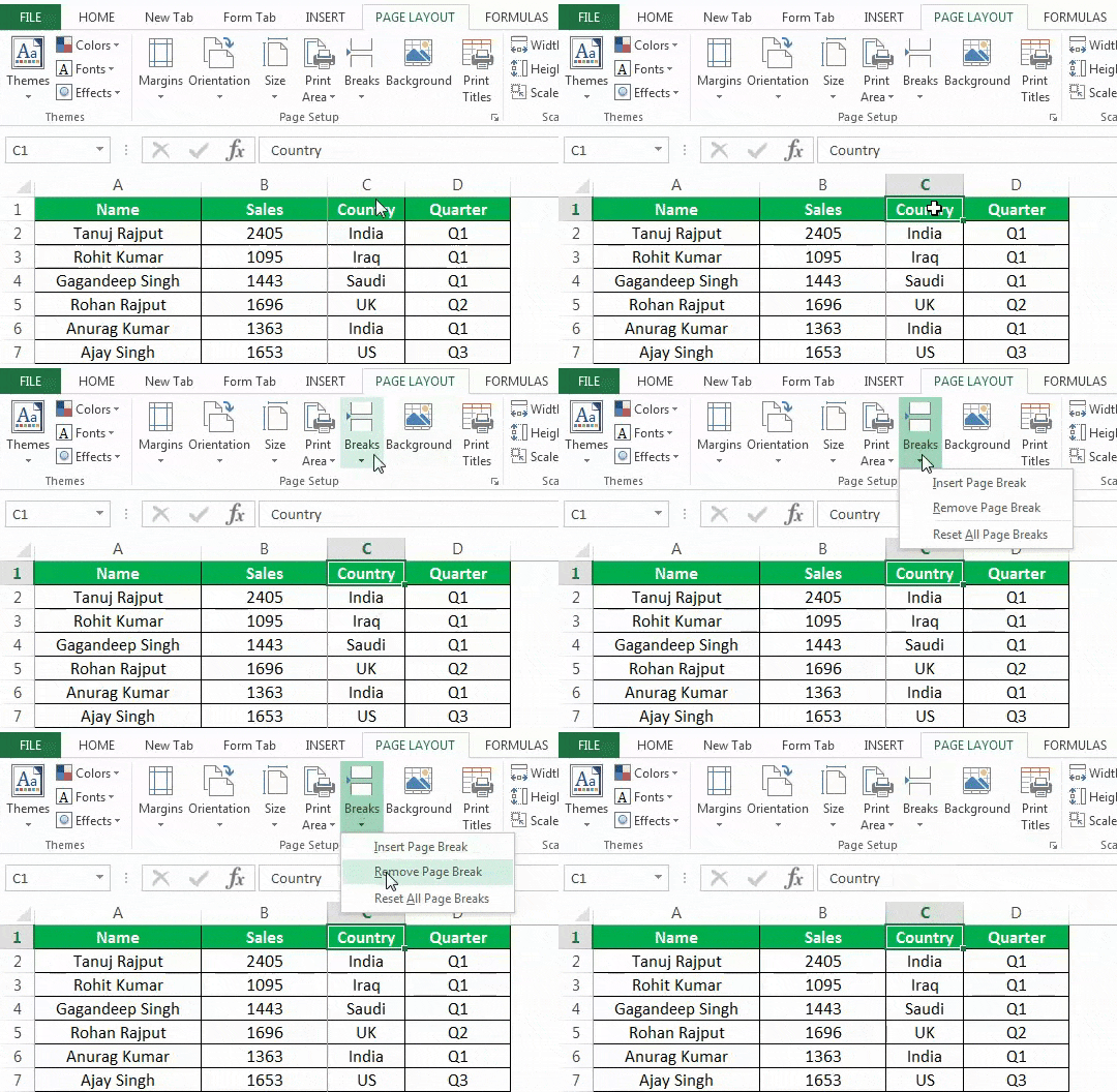
- Select the row or column of the Page Break to delete. Select the “Page Layout” tab, and click “Breaks”. Select “Remove Page Break”.
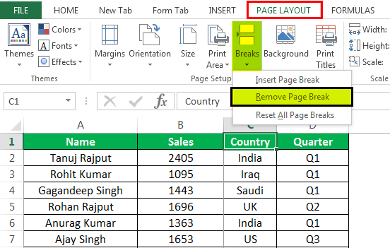
- It will delete the selected Page Break.
Important Things To Note
- It is a separator that breaks/divides an Excel worksheet into a separate page for printing.
- It is used to insert a Page Break in an Excel worksheet to specify where a new page will begin in the printed copy.
- We can enable or disable the “Show Page Break” option, to Show or Hide the Page Break, respectively, in the “File” tab.
Frequently Asked Questions (FAQs)
The steps to the Hide or Show Excel Page Break are as follows:
• 1: Select the “File” tab → click the “More” options → select the “Options”, as shown below.
• 2: The “Excel Options” window opens.
• The left, select the “Advanced” option.
• On the right, go to the “Display options for this worksheet:” category, check/tick the “Show Page Breaks” checkbox, to Show the Page Break, and click “OK”.
• Finally, on the right, go to the “Display options for this worksheet:” category, uncheck the “Show Page Breaks” checkbox, to hide the Page Break, and click “OK”, as shown below.
Instead of removing the Page Breaks vertically, horizontally, or cell by cell, we can remove all at once as follows:
Select the “Page Layout” tab → go to the “Page Setup” group → click the “Breaks” option drop-down → select the “Reset All Page Breaks” option, as shown below.
Therefore, we can delete all Page Breaks by clicking this option.
The keyboard shortcut key for inserting an Excel Page Break is,
.
The keyboard shortcut key for removing an Excel Page Break is,
.
The procedure to see if the Excel Page Break is applied correctly is,
Select the “View” tab → go to the “Workbook Views” group → click the “Page Break Preview” option, as shown below.
Then,the Page Break Preview feature will show the Page Break, represented by a blue highlighted outline.
A few reasons the Excel Page Break may not work are:
• It is applied on an empty worksheet, so the grey lines might be lightly visible giving the impression that there are no Page Breaks.
• They are not enabled. In such scenarios, we can go to the Excel Options window and enable/disable them to show/hide the page breaks, respectively.
Download Template
This article must help understand the Page Break in Excel with its features and examples. You can download the template here to use it instantly.
Recommended Articles
This article is a guide to Page Break in Excel. Here we learn to Move, Delete, Insert horizontal/vertical Page Break, examples & a downloadable excel template. You may learn more about Excel from the following articles: -
- Break in VBA
- Page Setup in Excel
- Line Breaks in Excel
- Week Number in Excel

