Table Of Contents
The Syntax of the OFFSET Excel Function
The syntax of the function is shown in the following image:

The function accepts the following mandatory arguments:
- Reference: This is the starting point from which the calculation of the ending cell (or range) address begins. It can be entered as a cell or a range of adjacent cells.
- Rows: This is the number of rows that the function needs to move. The movement can be either above or below the reference point (starting point). If this argument is positive, the function moves below the reference point. If this argument is negative, the function moves above the reference point.
- Cols: This is the number of columns that the function needs to move. The movement can be either to the right or the left of the reference point (starting point). If this argument is positive, the function moves to the right of the reference point. If this argument is negative, the function moves to the left of the reference point.
The function accepts the following optional arguments:
- Height: This is the height (number of rows) of the range to be returned.
- Width: This is the width (number of columns) of the range to be returned.
The “height” and the “width” arguments should always be positive numbers. If either of these arguments is omitted, the height and width of the reference (starting point) is assumed.
Note 1: The arguments “rows” and “cols” are specified using the reference point as the base.
Note 2: If both the “height” and “width” arguments are 1, the OFFSET excel function returns the value of a cell. This is because a 1-row by 1-column range is the dimension (size) of a single cell.
Note 3: The OFFSET function does not move any cell or range. It just returns the value of the cell (or range) address that it calculates.
How to use the OFFSET Function in Excel?
The OFFSET function is a built-in function of Excel. Let us understand its working with the help of a few examples.
Every example covers a different case of the OFFSET excel function, including an explanation of the same. In the last two examples (example #4 and #5), the OFFSET function has been combined with the arithmetic functions.
Example #1–End Point is a Data Cell
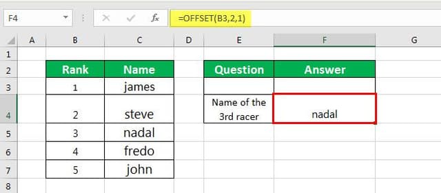
The following table shows the names of five racers and the corresponding ranks obtained by them. We want to find the name of the third racer with the help of the OFFSET function.
Step 1: Enter the following OFFSET formula in cell F4.
“=OFFSET(B3,2,1)”

Step 2: Press the “Enter” key. The output appears in cell F4. Hence, “Nadal” is the racer who ranked third in the race.

Explanation: The first argument of the OFFSET excel function is cell B3, which is the reference point (starting point).
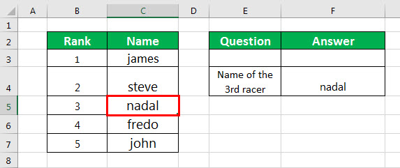
The “rows” argument is 2. So, the function moves two rows below cell B3, which is the cell B5. The “cols” argument is 1. So, the function moves one column to the right of cell B3, which is the cell C5.
The value of the resulting cell (end point) C5 is “Nadal.” Hence, the output in cell F4 is “Nadal.” The end point is shown in the following image.
Example #2–End Point is an Empty Cell
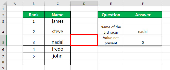
Working on the data of example #1, we want the OFFSET function to return the value of the empty cell D5.
Step 1: Enter the following formula in cell F5.
“=OFFSET(B3,2,2)”
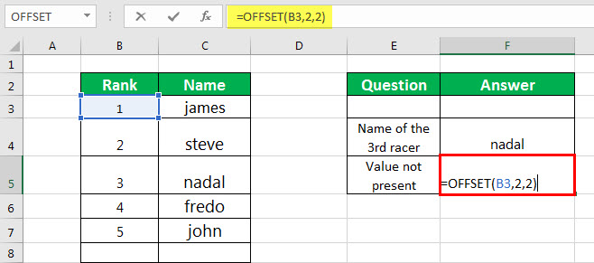
Step 2: Press the “Enter” key. The output 0 appears in cell F5. Hence, the OFFSET function returns the value of an empty cell as zero.
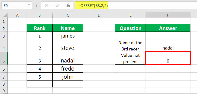
Explanation: In the given OFFSET excel formula, the reference point (starting point) is cell B3.
Since the “rows” argument is 2, the function moves two rows down to cell B5. The “cols” argument is also 2. So, the function moves two columns to the right of cell B3, which is the cell D5.
The resulting cell (end point) is D5. Since this cell is empty, the output returned by the OFFSET function is 0. The end point is shown in the following image.
Example #3–End Point is a Non-existent Cell
Working on the data of example #1, we want the OFFSET function to return the value of a cell (to the immediate left of cell A1) that does not exist.
Step 1: Enter the following OFFSET excel formula in cell F6.
“=OFFSET(B3,-2,-2)”
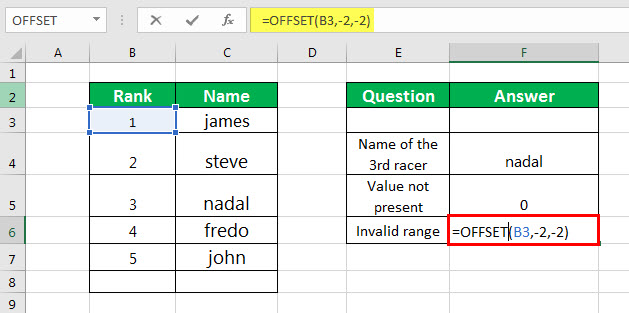
Step 2: Press the “Enter” key. The output appears in cell F6. Hence, the value of a non-existent cell is a “#REF!” error.
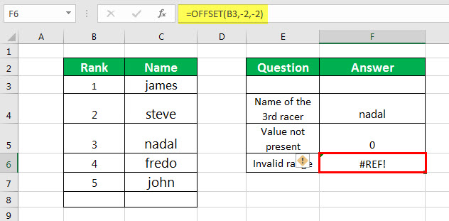
Explanation: In this example, cell B3 is the reference point.
The “rows” argument is -2. So, the function moves two rows above the cell B3, which is the cell B1. The “cols” argument is also -2. So, the function moves two columns to the left of cell B3. However, there is no column to the left of column A.
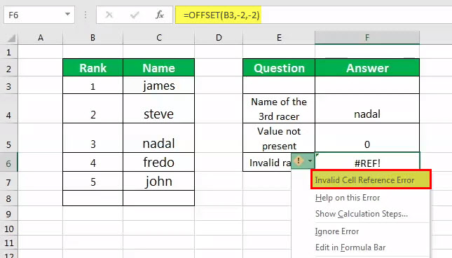
Hence, there is no resulting cell (end point). So, the output is “#REF!” error, as shown in the following image. The icon in yellow shows “invalid cell reference error.”
Note: If the end point of the OFFSET function is a cell which is out-of-range or non-existent, it returns a “#REF” error.
Example #4–Sum of Values of the Returned Range Address
The following table shows five stocks with their maximum and minimum returns (in $). We want to sum the maximum returns of these stocks. Use the OFFSET excel function combined with the SUM function.
Step 1: Enter the following formula in cell F3.
“=SUM(OFFSET(C2,0,0,5,1))”

Step 2: Press the “Enter” key. The output appears in cell F3. Hence, the sum of the maximum returns of the given stocks is $449.

Explanation: The cell C2 is the reference point.
Both the arguments “rows” and “columns” are zero. This implies that the OFFSET function will neither move up and down nor to the left and right.
The “height” argument is 5, implying that the OFFSET function will sum five rows beginning from the cell C2. This is the range C2:C6.
The “width” argument is 1, implying that the OFFSET function will sum the values of one column (column C).
With the given “height” and “width” arguments, the preceding formula (entered in step 1) returns the sum of values of a 5-row by 1-column range. It sums the values of the returned range (5-row by 1-column) because the OFFSET is enclosed within the SUM function.
Hence, the sum of all values of column C is calculated as 98+92+89+88+82=449.
Example #5–Average of Values of the Returned Range Address
Working on the data of example #4, we want to calculate the average returns of stock “S1.” Use the OFFSET excle function combined with the AVERAGE function.
Step 1: Enter the following formula in cell F5.
“=AVERAGE(OFFSET(C2,0,0,1,2))”

Step 2: Press the “Enter” key. The output appears in cell F5. Hence, the average return of stock “S1” is $74.

Explanation: The cell C2 is the reference point.
Both the arguments “rows” and “columns” are zero. This implies that the OFFSET function will not move in any direction.
The “height” argument is 1. This implies that the OFFSET function will consider only one row (row 2) for calculating the average.
The “width” argument is 2. This implies that the OFFSET excel function will calculate the average of two columns (columns C and D).
With the given “height” and “width” arguments, the preceding formula (entered in step 1) returns the average of a 1-row by 2-column range.
In the preceding formula, the OFFSET is enclosed within the AVERAGE function. So, the values of the returned range (1-row by 2-column) are used for calculating the average. Hence, the average of the values in the cells C2 and D2 is calculated as (98+50)/2=74.
Range Returned by the OFFSET Excel Function
The OFFSET function can also return the values of a range of adjacent cells. For this, the steps to be performed are listed as follows:
- Select a blank range of the size which is the same as specified by the “height” and “width” arguments of the OFFSET function in excel.
- Insert the OFFSET formula in the leftmost, top cell of the blank range.
- Press “Ctrl+Shift+Enter.” The curly brackets appear at the beginning and the end of the formula.
The values of the range of cells are obtained as the output of the OFFSET excel function.
Note: To obtain the values of a range of cells, it is essential to supply the “height” (number of rows) and “width” (number of columns) arguments.
