Normal Distribution

A normal distribution or Gaussian distribution refers to a probability distribution where the values of a random variable are distributed symmetrically. These values are equally distributed on the left and the right side of the central tendency. Thus, a bell-shaped curve is formed.

Also, the maximum number of values appears close to the mean; the tail consists of only a few values. The empirical rule applies to such probability functions. Therefore, 68% of the values lie within one standard deviation range. 95% of observations lie within two standard deviations, and 99.7% of the values appear within three standard deviations.

• A normal distribution is a statistical phenomenon representing a symmetric bell-shaped curve. Most values are located near the mean; also, only a few appear at the left and right tails.
• It follows the empirical rule or the 68-95-99.7 rule.
• Here, the mean, median, and mode are equal; the mean and standard deviation of the function are 0 and 1, respectively.
• This mathematical function has two key parameters:
  The mean (µ) and the standard deviation (σ).

A normal distribution resembles an asymmetric arrangement of most of the values around the mean, such that the curve so formed looks like a bell. It has two key parameters: the mean (µ) and the standard deviation (σ). This probability method plays a crucial role in asset return calculation and risk management strategy decisions. The following figure shows that the statistical probability function is a bell-shaped curve that follows the empirical rule:

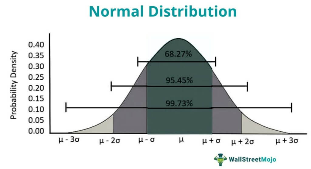
The possible outcomes of the function are given in terms of whole real numbers lying between -∞ to +∞. The tails of the bell curve extend on both sides of the chart (+/-) without limits.

1. Approximately 68% of all observations fall within +/- one standard deviation(σ).
2. About 95% of all observations fall within +/- two standard deviations (σ).
3. Nearly 99.7% of all observations fall within +/- three standard deviations (σ).

Skewness refers to symmetry. If skewness is 0, the data is perfectly symmetrical. If the normal distribution is uneven with a skewness greater than zero or positive skewness, then its right tail will be more prolonged than the left. Similarly, for negative skewness, the left tail will be longer than the right tail. Negative skewness means skewness is less than zero.

Kurtosis is a measure of peakiness. If the kurtosis is 3, the probability data is neither too peaked nor too thin at tails. If the kurtosis is more than three, then the data curve is heightened with fatter tails. Alternatively, if the kurtosis is less than three, then the represented data has thin tails with the peak point lower than the normal distribution. For a normal distribution, the kurtosis is 3.

Normal Distribution has the following characteristics that distinguish it from the other forms of probability representations:

• Empirical Rule: In a normal distribution, 68% of the observations are confined within -/+ one standard deviation, 95% of the values fall within -/+ two standard deviations, and almost 99.7% of values are confined to -/+ three standard deviations.
• Bell-shaped Curve: Most of the values lie at the center, and fewer values lie at the tail extremities. This results in a bell-shaped curve.
• Mean and Standard Deviation: This data representation is shaped by mean and standard deviation.
• Equal Central Tendencies: The mean, median, and mode of this data are equal.
• Symmetric: The normal distribution curve is centrally symmetric. Therefore, half of the values are to the left of the center, and the remaining values appear on the right. 
• Skewness and Kurtosis: Skewness is the the symmetry. The skewness for a normal distribution is zero. Kurtosis studies the tail of the represented data. For a normal distribution, the kurtosis is 3.
• Total Area = 1: The total value of the standard deviation, i.e., the complete area of the curve under this probability function, is one. Also, the entire mean is zero.

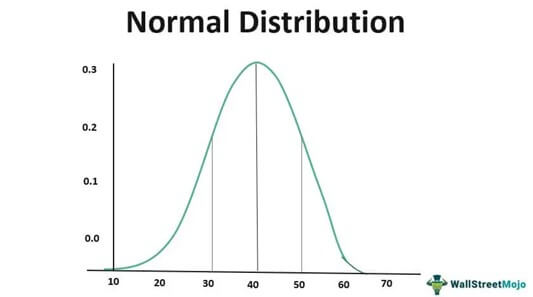
The curve takes the shape of a bell due to the symmetrical arrangement of the values that are concentrated towards the central tendency. At the same time, the tail consists of an insignificant number of values.

Have a look at the curve below to understand its shape better:

The Probability Density Function (PDF) of a random variable (X) is given by:

Where;

• -∞ < x < ∞; -∞ < µ < ∞; σ > 0
• F(x) = Normal probability Function
• x = Random variable
• µ = Mean of distribution
• σ = Standard deviation
• of the distribution
• π = 3.14159
• e = 2.71828

Transformation (Z)

When it comes to a comparative study of two or more samples, there arises a need for converting their values in z-scores. This is termed as z-transform.

Transformation Formula

For ascertaining the z-score, the following formula is used:

Where X = Random variable.

Normal Distribution Table

The table referred for the standard deviation is the z-table. Here, we determine the probability of getting a particular outcome using the transformation formula to ascertain the value of the z-score, which is depicted in percentage using a z-table.

Example #1

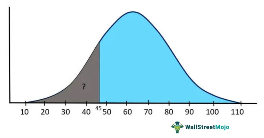
Let us suppose that a company has 10000 employees and multiple salary structures according to specific job roles. The salaries are generally distributed with the population mean of µ = $60,000, and the population standard deviation σ = $15000. What will be the probability of a randomly selected employee earning less than $45000 per annum?

Solution:

As shown in the above figure, we need to find out the area under the normal curve from 45 to the left side tail to answer this question. Also, we need to use the z-table value to get the correct answer.

Firstly, we need to convert the given mean and standard deviation into a standard normal distribution with mean (µ)= 0 and standard deviation (σ) =1 using the transformation formula.

After the conversion, we need to look up the z-table to find out the corresponding value, which will give us the correct answer.

Given,

• Mean (µ) = $60,000
• Standard deviation (σ) = $15000
• Random Variable (x) = $45000

Transformation (z) = (45000 – 60000 / 15000)

Transformation (z) = -1

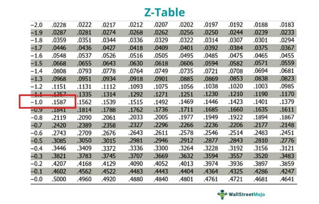
The value equivalent to -1 in the z-table is 0.1587, representing the area under the curve from 45 to the left. Thus, it indicated that when we randomly select an employee, the probability of making less than $45000 a year is 15.87%.

It is important to note that we have converted the z-score value 0.1587 into a percentage by multiplying it by 100 to get 15.87%.

Example #2

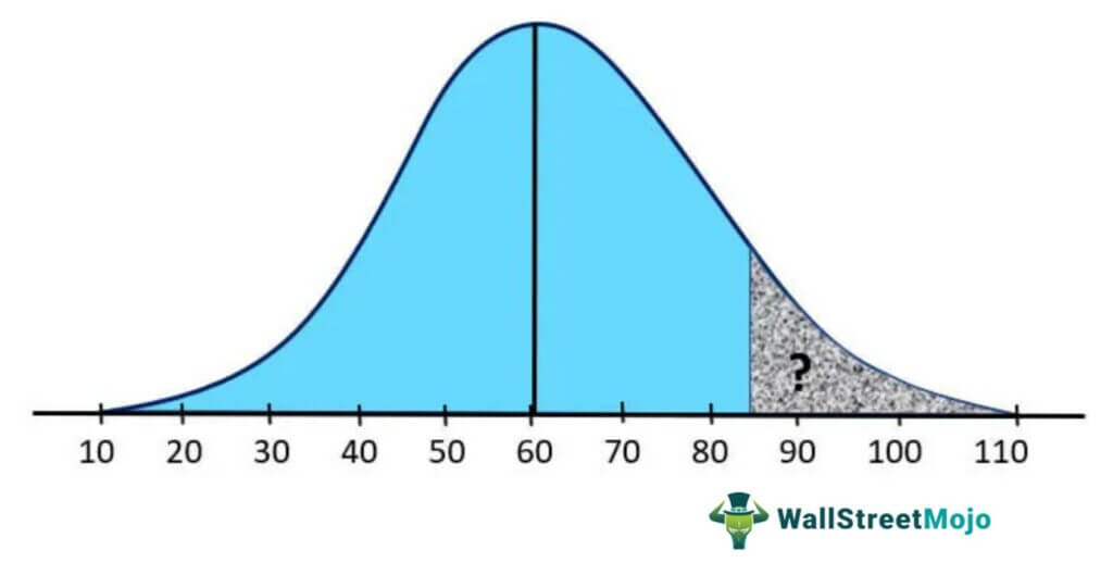
For the same above scenario, now find the probability of a randomly selected employee earning more than $85,000 a year.

Solution:

So, in this question, we need to find out the shaded area from 85 to right tail using the same formula.

Given:

• Mean (µ) = $60,000
• Standard deviation (σ) = $15000
• Random Variable (X) = $85,000

Transformation (z) = (85000 – 60000 /15000)

Transformation (z) = 1.67

As per the Z-table, the equivalent value of 1.67 is 0.9525 or 95.25%, which shows that the probability of randomly selecting an employee earning less than $85,000 per annum is 95.25%.

But as per the question, we need to determine the probability of random employees earning more than $85,000 a year, so we need to subtract the calculated value from 100.

• Random Variable (X) = 100% – 95.25%
• Random Variable (X) = 4.75%

So, the probability that employees earn more than $85,000 per year is 4.75%.

This mathematical function is applied in various fields of study, whether it is science, economics, statistics, finance, business, investment, psychology, health, genetics, biotech, or academics. Some of its typical applications are discussed below:

• The stock market technical chart is often a bell curve, allowing analysts and investors to make statistical inferences about stocks' expected return and risk.
• It is used to determine pizza companies' best time to deliver pizza and similar real life applications.
• It is also applied in business operations to determine the efficiency of products, resources, and sales.
• It is used in comparing the heights of a given population set in which most people will have average heights. Very few people will have above average or below average height.
• They are used in determining the average academic performance of students. This mathematical function is used in determining the rank of a student.

The Gaussian Function is commonly used in data science and data analytics. Advanced technologies like artificial intelligence (AI) and machine learning can deliver better results when used along with normal density functions.

This has been a guide to Normal Distribution in Statistics and its definition. Here we explain its characteristics along with its formulas, examples and uses. You can learn more about financing from the following articles –

• NORMDIST Excel
• Log Normal Distribution
• Formula of Normal Distribution
• Create Normal Distribution Graph in Excel