Table Of Contents
Excel Negative Numbers
Microsoft Excel uses positive and negative numbers in performing mathematical calculations. In Excel, negative numbers are displayed with minus symbols by default. These are the numbers that are lower than 0 in value. Excel makes it easy to recognize the negative numbers by facilitating various best practices.
It needs to recognize the negative numbers while performing the calculations. In some scenarios, such as determining variance, it is necessary to convert the negative numbers to positive numbers or represent them in an appropriate format to use the negative values appropriately. It is required to represent them by applying a specific conditional format based on the requirement.
The present article aims to identify ways to manage the negative numbers in Excel.
Explanation of Negative Numbers in Excel
Handling the negative numbers is very easy in Excel. Excel can manage both positive and negative numbers effectively. But, negative numbers can generate some confusion for the users sometimes. There is a chance for the occurrence of issues while handling negative numbers when the inappropriate format is chosen for them. It displays the errors when a user tries to perform calculations on the negatives.
Entering the negative numbers with a minus sign is very easy but analyzing them is tough when a mixture of positive and negative values is presented. To avoid this problem, it needs to change the format of the Excel cells that contain negative values to get accurate results.
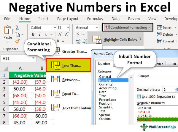
How to Show Negative Numbers in Excel?
Negative numbers have a lot of significance in handling the various applications in Excel. Therefore, applying the set of formats is important in multiple areas.
- Financial analysts use a best practice in financial modeling representing the negative values in red.
- Negative numbers are squared in the determination of variance in data analysis to remove the problem presented with standard deviation.
- When the variance value is negative, it is multiplied by -1 to make it positive.
- In VBA, negative numbers represent the dates before the 1900 year.
- When we need the only absolute value of the negative number, the absolute function is applied to get a positive value.
Top 3 Ways to Show/Highlight Negative Numbers in Excel
This section will describe the various ways to show/highlight negative numbers in Excel.
Example#1 - With Conditional Formatting
Representing negative numbers with conditional formatting
This example illustrates the Excel conditional formatting to highlight the negative numbers in various steps. For this example, we need to use numbers that are lower than 0.
The following data is considered to illustrate this example.
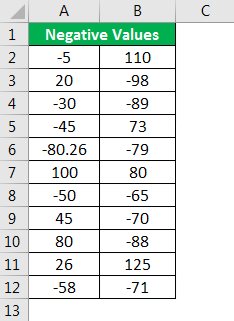
Step 1: We must first select the entire range of data as shown in the figure.
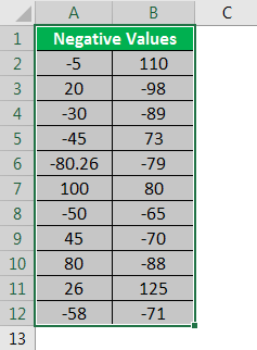
Then, go to the "Home" tab and select conditional formatting. Next, select the "Highlight Cells Rules" and "Less Than" under the options presented.
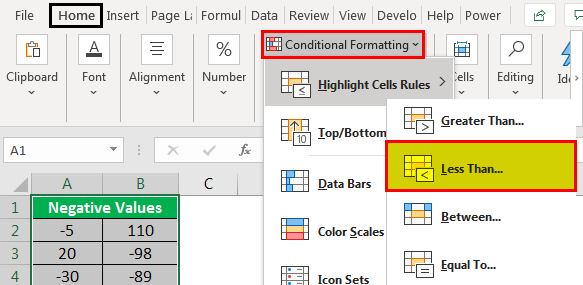
It opens the "Less Than" dialog box, as shown in the figure.

Step 2: Enter the value in the empty box under "Format cells that are LESS THAN" and click on the dropdown right to "with’ to apply the desired formatting to the numbers. Ensure that "Light Red Fill with Dark Red Text" is highlighted. Then click on "OK."

The output is shown as,
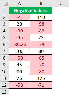
The above figure identifies that the cells with values less than 0 are highlighted with a red fill and red color to text. This type of conditional formatting is also applied with greater than, between, equal to, and duplicate values with negative values.
Example#2 - With Inbuilt Number Formatting
Representing negative numbers with inbuilt number formatting
This example is to illustrate the Excel inbuilt number formatting to highlight the negative numbers in red color. For this example, we need to use numbers that are lower than 0. The following are the steps required
The following data is considered to illustrate this example.
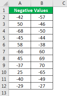
Step 1: Select the data that you want to apply the inbuilt custom formatting with a red color.
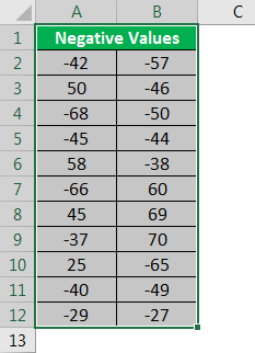
Step 2:
- Go to the "Home" tab.
- Click on "Number Format."
- Click on the small tilted icon on the right side corner.
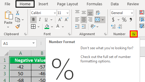
It helps in opening the "Format Cells" dialog box.
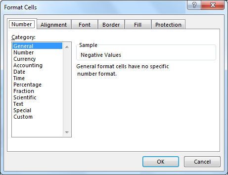
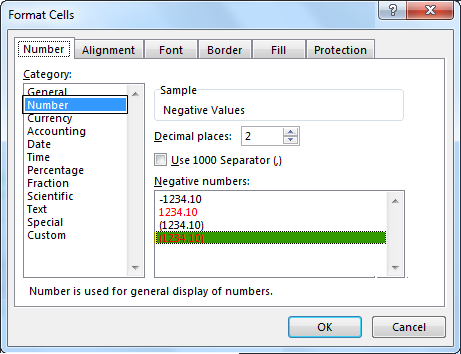
Step 3: In the "Format Cells" dialog box, ensure that the "Number" tab is highlighted in the "Format Cells" dialog box. Go to "Number" under the "Number" tab. Select the red text option with brackets for negative numbers on the right side of the options. And click on "OK."
Step 4: The formatted Excel negative numbers will look as follows,
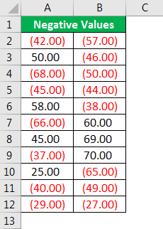
Two decimal points are automatically added to numbers when the formatting is applied.
Example#3 - With Custom Number Formatting
Representing negative numbers with custom number formatting
This example illustrates the custom number formatting to highlight the negative numbers in Excel. For this example, we need to use the numbers which are lower than 0.
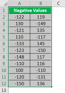
The following data is considered to illustrate this example.
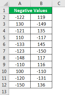
Step 1: We must select the data that we want to apply the inbuilt custom formatting with a red color.
Step 2: Go to the "Home" tab.
- Click on "Number format’."
- Click on the small tilted icon on the right side.
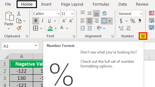
It helps in opening the "Format Cells" dialog box.

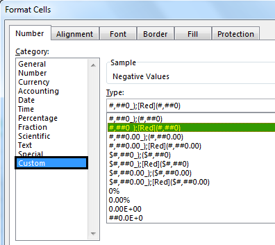
Step 3: The dialog box ensures that the "Number" tab is highlighted in the "Format Cells." Go to the "Custom" option under the "Number" tab. Select the appropriate format, as shown in the figure. Click on "OK" to apply the formatting.
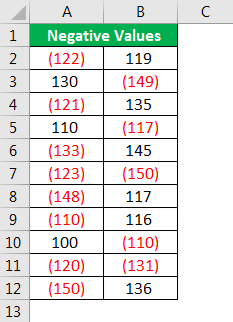
Step 4: The negative numbers will look as follows in Excel.
Things to Remember
- Conditional formatting is volatile. Whenever values change in the Excel sheet, it reassesses the condition and changes the formatting of the dataset. Therefore, it will become a problem for large datasets.
- We can apply any color to the background and text in Excel cells to highlight the negative numbers.

