Name Box in Excel

What is Name Box in Excel?

Name box in excel is located on the left side of the excel window and it used to give a name to a table or any cell, for any normal cells by default the name is the row character and the column number such as cell A1, we can check it when we click on the cell it shows in the name box as A1 but we can input any name for the cell and press enter and refer to the cell with the name we put in the name box.

Name Box is a tool that shows the active cell address. For example, if you have selected the cell C1, this name box will show the active cell address as C1.

• The first scenario in excel is when we are working with excel by mistake, we would press some other key from the keyboard, and suddenly our active cell goes missing, and we don’t know what is the active cell now. How do you find what is the active cell now?
• The second one is I have seen most of the people use a range of cells as reference for their formulas when we can use named ranges easily without worrying about the wrong range of cells selection and finding the range of cells in the large worksheet.

Both of the above seems like bigger problems, but solutions are as simple as it gets. The solution for both scenarios is “Name Box.” In this article, we will take you through the tool Name Box.

Where to Find Name Box in Excel?

The name box is available at the left end of the formula bar in excel. Even though we work enough time with excel spreadsheets, it goes unnoticed by many of the users.

How to Use Name Box in Excel?

The usage of Name Box is not only limited to active cell address, but it has a lot more features which can be critical in usage on a daily basis. Now we will see what the usage of this name box is.

#1 – Quick & Fast to go to the Specific Cell

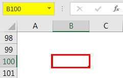
This is one of the great features because when we work with large databases often times, we need to go back to the specific cells to do the job. For example, assume you want to go to the cell B100; it will take a hell of a lot of time to reach that cell if you are scrolling down the worksheet. But using Name Box, we can quickly locate the cell and reach that cell.

• Step 1: For this, first select the Name Box.

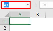
• Step 2: Now type the cell address that you want to go to.

• Step 3: After typing the desired cell address, hit the enter key; it will take you to the mentioned cell.

#2 – Select More than Once Cell at a Time

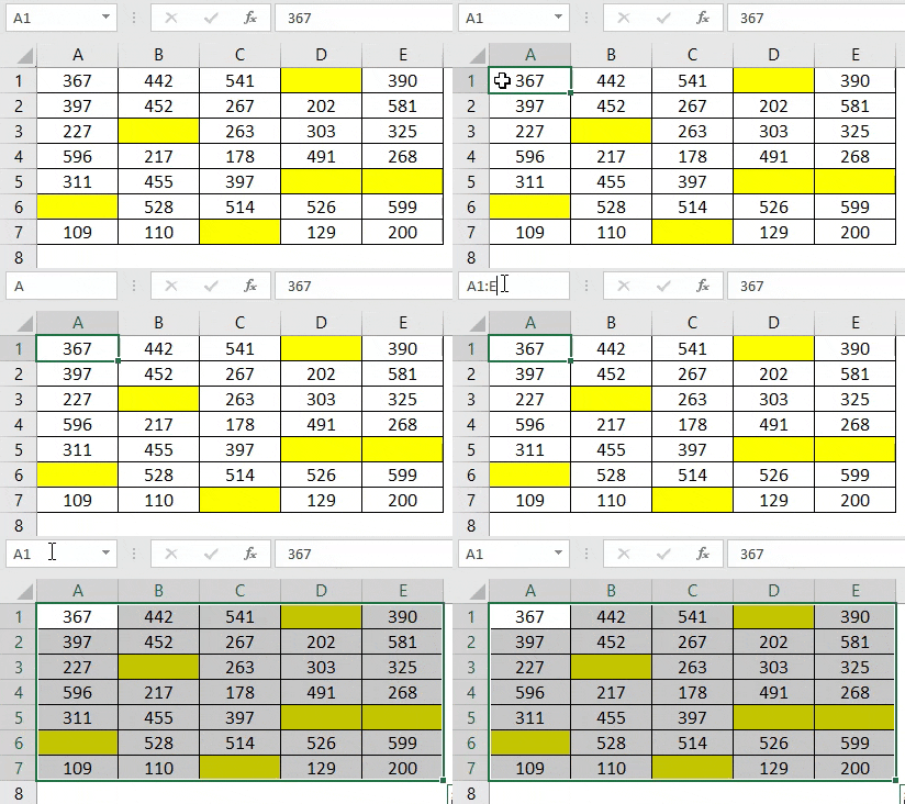
Assume you have data like the below picture.

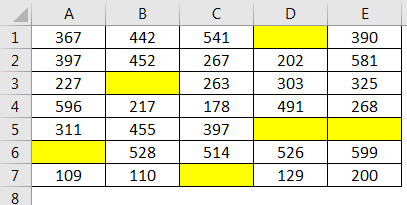
 In this data, we have blank cells; if we want to select the full data range, if we use shortcut key Shift + Ctrl + Right Arrow from cell A1, it will only select until it finds the blank cell, i.e., until cell D1.

Similarly, for the shortcut key Shift + Ctrl + Down Arrow, it will stop at the A6 cell.

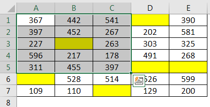
In such cases, the more blanks cells and the more time it takes and frustrating because of irritating blank cells. To quickly select this range of cells, we can enter the range of cells in the name box itself.

In this case, our first cell to be selected is A1, and the last cell is E7. So type the range of cell address as A1:E7 in the name box, then hit the enter key; it will select the mentioned range of cells quickly.

#3 – Select Range of Cells From Active Cell

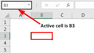
Assume your active cell right now is B3, and from this cell, you want to select the range of cells as B3:D6.

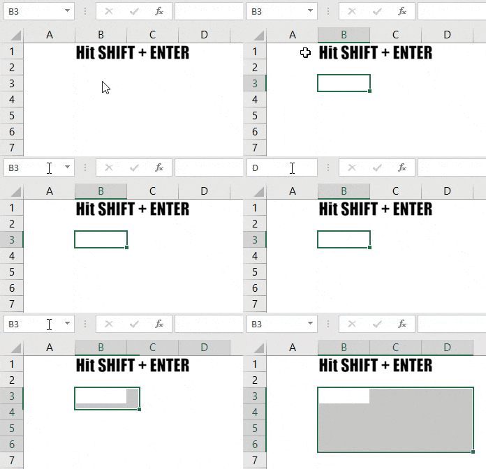
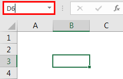
We need not mention the range of cells as B3:D6 rather from active cell enter the end of the range of cell address. Now, in the name box, type the last cell to be selected, i.e., D6 cell.

Now simply don’t hit the enter key; rather, hit the Shift + Enter key to select the range of cells.

#4 – Select only Two cells

In the above example, we have selected a range of cells. From active cell B3, we have entered D6 as the last cell of the range and hit Shift + Enter to select the range as B3 to D6, but instead of pressing Shift + Enter, if we press Ctrl + Enter, it will select only two cells, i.e., B3 & D6.

Now hit Ctrl + Enter to select two cells, i.e., B3 & D6.

#5 – Select Multiple Range of Cells

In the above two examples, we have seen how to select a range of cells from active cell and two individual cells. Now we will see how to select multiple ranges of cells. For example, look at the below data.

In the above image, we have two sets of ranges one is from A1 to C5, and another one is from E1 to F5. We can select two different range of cells from the name box. Enter two range of cells separated by comma (,).

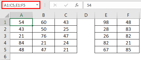
After entering the range, address hit the enter key or Ctrl + Enter to select the range of cells as mentioned.

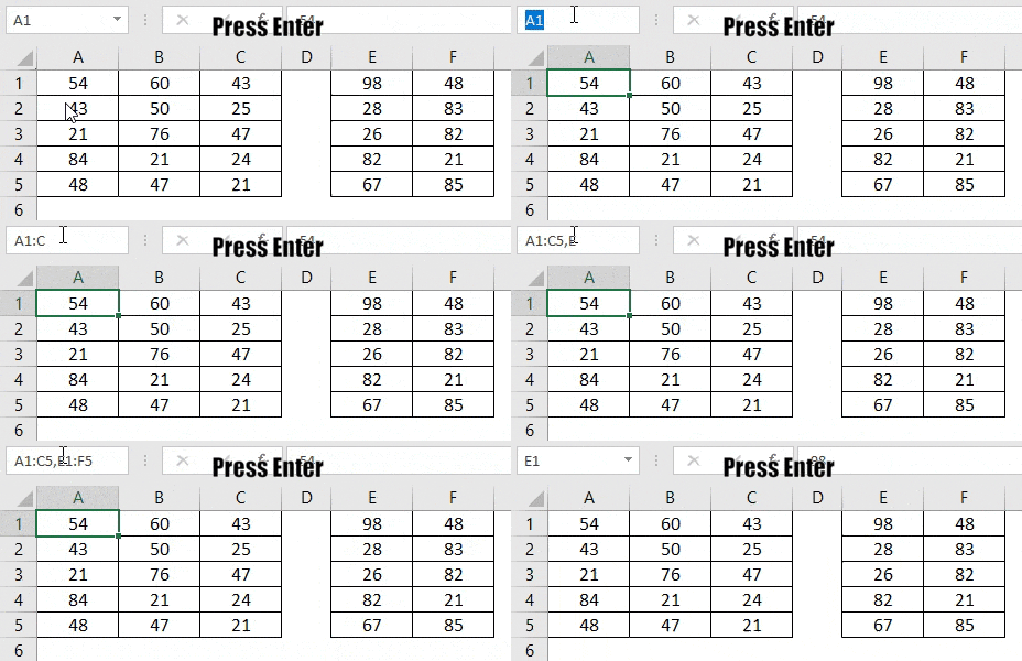
#6 – Select Entire Column

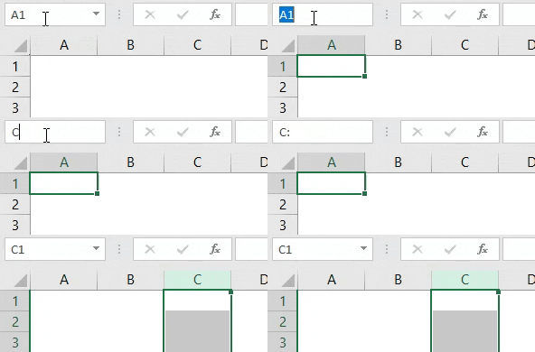
We can also select the entire column from the name box. For example, if we want to select the entire column C, then type the address as C:C.

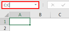
Hit the enter key after you mention the column address.

#7 – Select Entire Row

We can also select the entire row from the name box. For example, if we want to select the entire row 2, then type the address as 2:2.

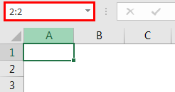
Hit the enter key after you mention the row address.

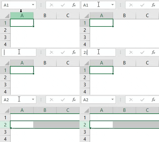
Like this, we can use excel Name Box to our advantage at our workplace to work efficiently.

Recommended Articles

This has been a guide to Name Box in Excel. Here we discuss how to use the name box property to find the active cell address and to select the entire range of cells, rows & columns in excel along with practical examples and a downloadable excel template. You may learn more about excel from the following articles –

• Compare and Match Excel Columns
• Excel AVERAGEIFS Function
• What is Excel Dynamic Named Range?
• Name Range in Excel
• Row Limit in Excel