NA Excel

What Is NA Excel?

The NA Excel function is an inbuilt Information function. It returns the #N/A error value, which indicates a cell with no data. While the function is an alternative for typing the error value directly into a cell, it provides compatibility with other spreadsheet applications.

Users can utilize the NA Excel function to highlight cells that are missing data in a worksheet and exclude empty cells from financial and statistical Excel calculations.

For example, the following dataset contains a list of items and their sales data.

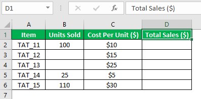
The aim is to find the total sales figures of each item based on their units sold and cost per unit data and display the output in column D.

But the output must show the #N/A error value if the units sold data for the particular item is unavailable.

Then, we can use the IF NA Excel functions-based formula in each target cell to achieve the required data.

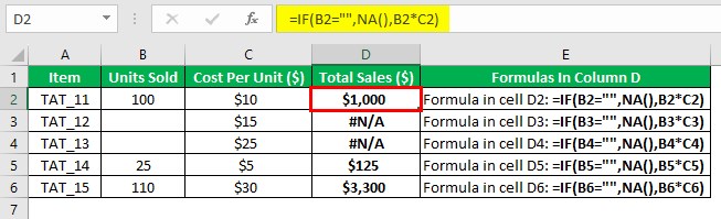
In the above NA Excel formula example, the Excel IF function in each target cell checks if the corresponding column B cell is empty.

If the specified column B cell is empty, the IF() condition holds, leading to the NA Excel function returning the #N/A error value as the IF() output. Otherwise, the formula multiplies the corresponding units sold and cost per unit values to return the total sales figure of the specific item as the IF() output.

• The NA Excel function is an inbuilt function that returns the #N/A error value as the output. It is an alternative for typing the #N/A error value in a chosen cell.
• Users can utilize the NA function in a cell to indicate the specific cell does not contain data. Also, it helps users to ignore empty cells while performing calculations in Excel.
• We can enter the NA function directly into a cell or from the Formulas tab. On the other hand, the function does not take any arguments.
• While we can utilize the NA function as a standalone function, using it with other inbuilt functions, such as IF and VLOOKUP, yields practical outcomes.

Syntax

The NA Excel function syntax is as follows:

The NA Excel formula does not take any arguments.

How To Use NA Excel?

We can utilize the NA Excel function in two ways, namely,

1. Access from the Excel ribbon.
2. Enter into the worksheet manually.

Method #1 – Access From The Excel Ribbon

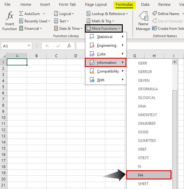
Choose a target cell for output - select the Formulas tab - click the More Functions option down arrow - click the Information option right arrow - choose the NA Excel function, as depicted below.

The Function Arguments window will open. However, since the NA Excel function does not accept any arguments, the Function Arguments window shows the function output.

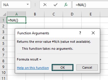
Click OK in the Function Arguments window to close it and view the #N/A error in the target cell.

Method #2 – Enter Into The Worksheet Manually

1. Choose a target cell for the output.
2. Type =NA( in the cell.
3. Close the brackets and press Enter to view the #N/A error value in the target cell.

Examples

Check out the following NA Excel function examples to use it effectively.

Example #1

Let us see an IF NA Excel functions-based formula example.

The following dataset contains employees, their annual salaries and expected incentives.

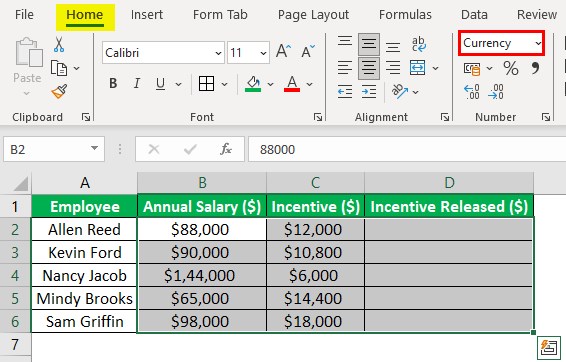
The aim is to update the incentive released data for each employee in column D based on their annual salaries and incentive figures. Assume the condition to release the incentive is that an employee’s annual salary must be less than $70,000 or greater than or equal to $100,000.

Further, the cell range B2:D6 has the same data format Currency.

Then, here is how to use the IF and NA Excel functions-based formula in the target cells to achieve the required outcome.

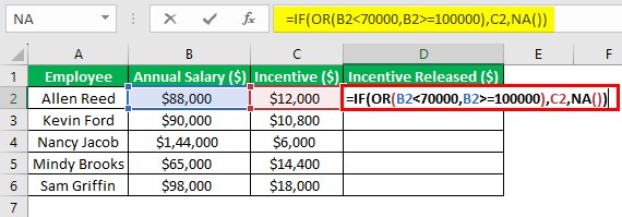
Step 1: Choose cell D2 and enter the IF() containing the NA Excel function.

=IF(OR(B2<70000,B2>=100000),C2,NA())

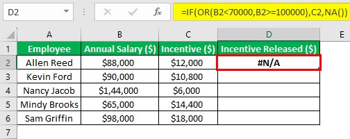
Step 2: Press Enter to view the formula output.

Step 3: Using the Excel fill handle, update the formula in the remaining target cells.

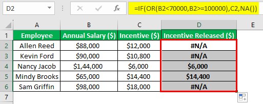
Let us check the cell D6 formula to understand the logic.

First, the Excel OR function, specified as the IF() condition, checks if the salary amount in cell B6 is less than $70,000 or greater than or equal to $100,000. As the salary figure in cell B6 does not meet any of the conditions in the OR(), the IF() condition does not hold.

Thus, the FALSE value, NA(), gets executed, leading to the IF() returning the NA() output, the #N/A error value, as the output.

Example #2

We shall see an example of sum if not NA Excel.

The following dataset contains a list of branch offices and their monthly sales figures from Jan-Mar.

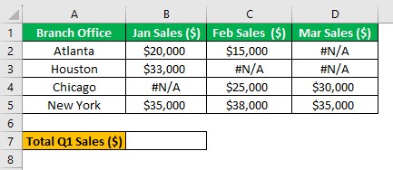
The aim is to add the monthly sales data of all branch offices and display the output in cell B7 as the total Q1 sales, provided the source dataset does not have the #N/A error value. Otherwise, the output in the target cell should be the #N/A error value.

Step 1: Choose cell B7 and enter the Excel SUM function containing the NA Excel function.

=SUM(IF(ISNA(B2:D5),NA(),B2:D5))

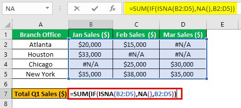
Next, press Ctrl + Shift + Enter to execute the expression as we would to implement array formulas in Excel.

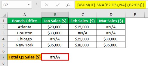
First, the ISNA Excel function returns an array of TRUEs and FALSEs based on whether the corresponding data point is the #N/A error value or a valid value in the cell range B2:D5.

Next, since the ISNA() output is the IF() condition, the IF() output will be an array of valid numbers and the #N/A errors. While the TRUEs will get updated as the #N/A error value, the FALSEs will get updated as the valid values in the cell range B2:D5.

Finally, the SUM() adds the array values, which are the numbers and the #N/A error, leading to the #N/A error as the required total Q1 sales figure. The reason is that the array of values to add contains the #N/A error value, and the function determines the sum if not NA Excel in the specified range.

Thus, if the range B2:D5 contained only valid numbers or the formula had a 0 as the TRUE value instead of the NA Excel function, the SUM() output would be a valid number.

Example #3

Let us see an example of the NA Excel function in the VLOOKUP Excel function.

The following dataset contains a list of fruits and their order details.

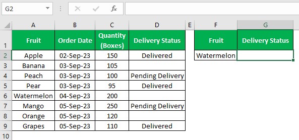
The aim is to determine the delivery status of the fruit specified in cell F2 based on the source dataset. If the required data is not in the source dataset, the output must show the #N/A error value. Otherwise, the output should be the fruit's delivery status based on the source dataset. Assume the target cell is G2.

Then, we can utilize the NA Excel VLOOKUP function-based formula in the target cell to achieve the required output.

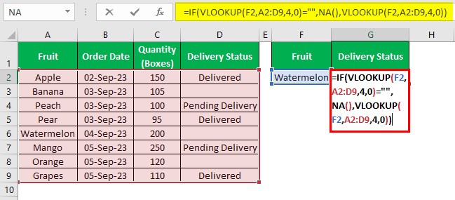
Step 1: Choose cell G2 and enter the VLOOKUP() containing the NA Excel function.

=IF(VLOOKUP(F2,A2:D9,4,0)="",NA(),VLOOKUP(F2,A2:D9,4,0))

Step 2: Press Enter to execute the NA Excel VLOOKUP function-based formula.

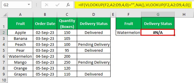
First, the IF() condition is a VLOOKUP(). It checks for the fruit specified in cell F2 in the first column of the lookup range A2:D9. It finds the fruit in cell A6. Thus, the VLOOKUP() output is the return value in the corresponding column D row, the cell D6.

However, cell D6 is empty. Thus, the IF() holds, and the TRUE value, NA(), gets executed to return the #N/A error value as the IF() output in the target cell.

Important Things To Note

• Ensure to include an empty parenthesis when using the NA Excel function. Otherwise, Excel will not recognize the entry as a function.
• The NA function offers compatibility with other spreadsheet-based programs.
• If a formula refers to a cell or range containing the #N/A error value, its return value will be the #N/A error value.

Frequently Asked Questions (FAQs)

Download Template

This article must be helpful to understand the NA Excel, with its formula and examples. You can download the template here to use it instantly.

Recommended Articles

This article is a guide to What Is NA Excel. Here we explain the NA function syntax and different ways to use it in Excel with examples and points to remember. You can learn more about Excel functions from the following articles: –

• #Div/0! Excel Error
• IFERROR Excel Function
• #VALUE! Error in Excel