Table Of Contents
MONTH Function in Excel
The MONTH function in Excel is a date function used to find the month for a given date in a date format. This function takes an argument in a date format, and the result is in integer format. This function's value is in the range of 1-12 as there are only twelve months in a year. The method to use this function is as follows =MONTH( serial_number). The argument provided to this function should be in a recognizable date format of Excel.
For example, =MONTH(A1) - returns the month of a date in A1.
=MONTH(DATE(2020,6,10)) - returns 6 corresponding to June.
Also, =MONTH("10-June-2020") - returns number 6 too.
The MONTH function in Excel gives the month from its date. It returns the month number ranging from 1 to 12.
MONTH Formula in Excel
Below is the MONTH Formula in Excel.

Or
MONTH( date )
MONTH in Excel - Illustration
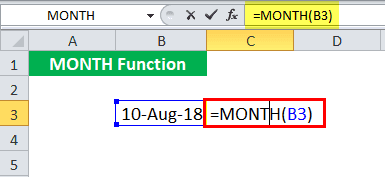
Suppose a date (10 August, 18) is given in cell B3. You want to find the month in Excel of the given date in numbers.
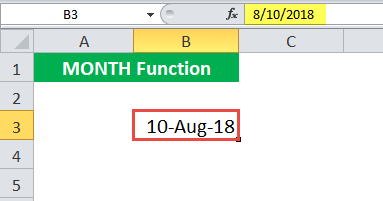
You can use the MONTH formula in Excel given below:
= MONTH (B3)

Press the "Enter" key. The MONTH function in Excel will return 8.
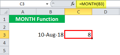
You can also use the following MONTH formula in Excel:
= MONTH (“10 Aug 2018”)
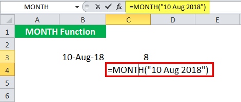
Press the "Enter" key. The MONTH function will also return the same value.
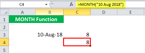
The date 10 Aug 2018 refers to a value 43322 in Excel. You can also use this value directly as input to the MONTH function. The MONTH formula in Excel would be:
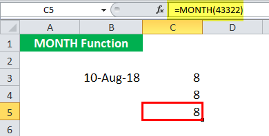
= MONTH (43322)
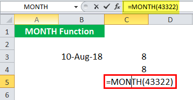
MONTH function in Excel will return 8.
Alternatively, you can also use the date in another format:
= MONTH (“10-Aug-2018”)
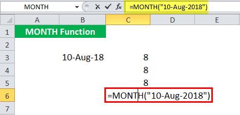
Excel MONTH function will also return 8.
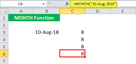
Let us look at examples of where and how to use the MONTH function in Excel in various scenarios.
Video Explanation of MONTH Excel Function
How to Use MONTH Function in Excel?
The MONTH function in Excel is very simple and easy to use. Let us understand the working of a MONTH in excel by some examples.
serial_number: a valid date for which the month number is to be identified
The input date must be a valid Excel date. The dates in Excel are stored as serial numbers. For example, the date Jan 1, 2010, equals the serial number 40179 in Excel. The MONTH formula in Excel takes as input both the date directly or the serial number of the date. It is to be noted here that Excel does not recognize dates earlier than 1/1/1900.
Returns
The MONTH function in Excel always returns a number ranging from 1 to 12. This number corresponds to the month of the input date.
MONTH in Excel Example #1
Suppose you have a list of dates given in the cells B3: B7, as shown below. You want to find the month name of each of these given dates.
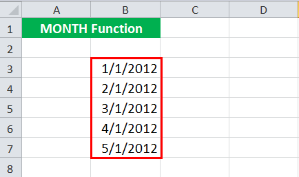
You can do so using the following MONTH formula in Excel:
= CHOOSE ((MONTH(B3)), “Jan”, “Feb”, “Mar”, “Apr”, “May”, “Jun”, “Jul”, “Aug”, “Sep”, “Oct”, “Nov”, “Dec”)
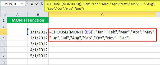
MONTH (B3) will return 1.
CHOOSE (1, …..) will choose the 1st option of the given 12, Jan here.
So, the MONTH function in Excel will return Jan as a result.
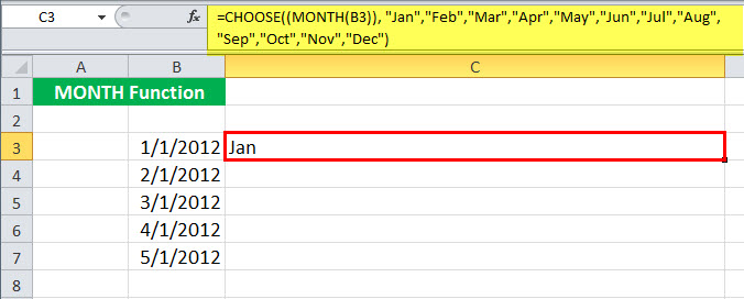
Similarly, you can drag it for the rest of the cells.
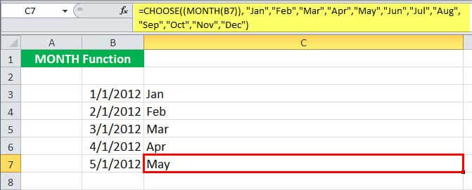
Alternatively, you can use the following MONTH formula in Excel:
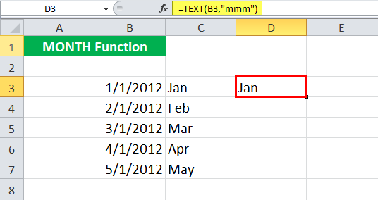
= TEXT (B3, “mmm”)
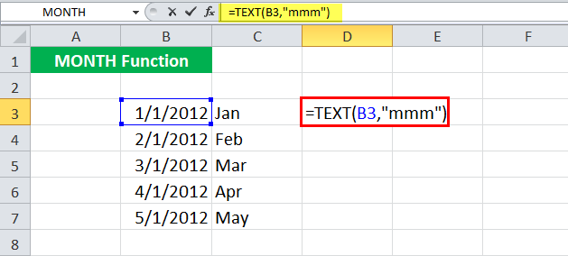
The MONTH function will return Jan as a result.
MONTH in Excel Example #2
Suppose you have month names (say in “mmm” format) given in cells B4: B15.
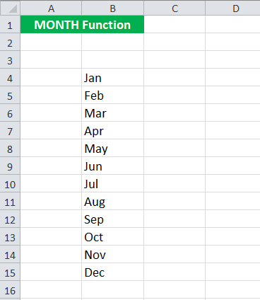
Now, you want to convert these names to the month in numbers.
You can use the following MONTH in Excel:
= MONTH ( DATEVALUE( B4 & ” 1”)
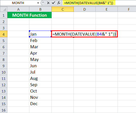
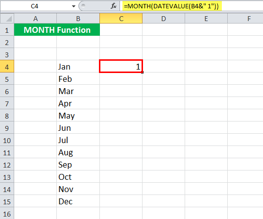
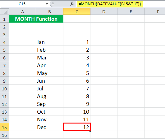
For Jan, the MONTH in Excel will return 1. For Feb, it will return 2 and so on.
MONTH in Excel Example #3
Suppose you have a list of holidays given in cells B3: B9 in a date-wise manner, as shown below.
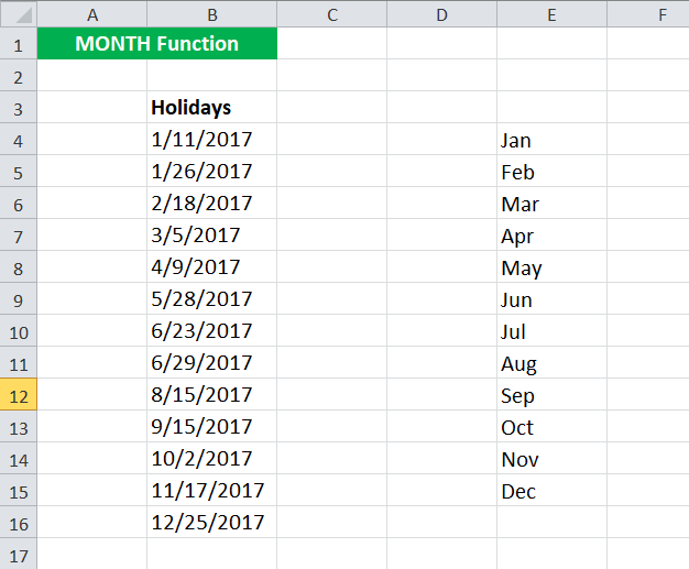
Now, you want to calculate the number of holidays each month. To do so, you can use the following MONTH formula in Excel for the first month given in E4:
= SUMPRODUCT( --( MONTH( $B$4:$B$16 ) = MONTH( DATEVALUE( E4 & " 1")) ) )
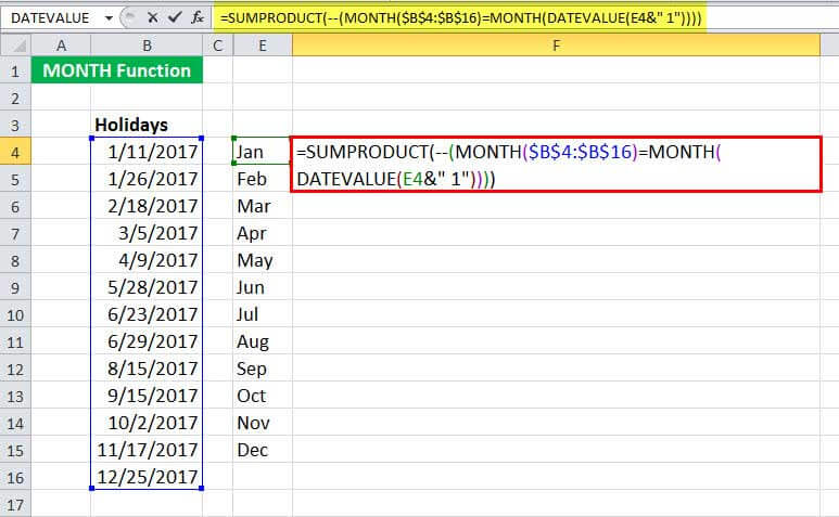
Then, drag it to the rest of the cells.
Let us look at the MONTH function in Excel detail:
- MONTH( $B$4:$B$16 ) will check the month of the dates provided in cell range B4:B16 in a number format. The MONTH function in Excel will return {1; 1; 2; 3; 4; 5; 6; 6; 8; 9; 10; 11; 12}
- MONTH( DATEVALUE( E4 & ” 1″) will give the month in number corresponding to cell E4 (see example 2). The MONTH function in Excel will return 1 for January
- SUMPRODUCT in Excel (– (…) = (..) ) will match the month given in B4:B16 with January (=1) and will add one each time when it is true.
Since January appears twice in the given data, the MONTH function in Excel will return 2.
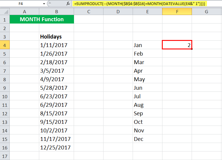
Similarly, you can do for the rest of the cells.
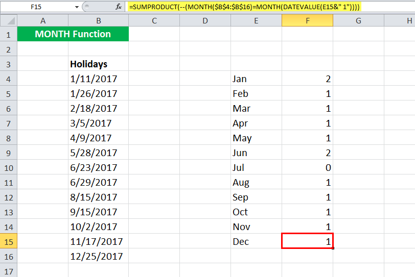
MONTH in Excel Example #4
Suppose you have sales data for the past two years. The data was collected on the last date of the month. The data was manually entered, so there could be a mismatch in the data. You should compare the sales between 2016 and 2017 for each month.
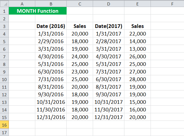
To check if the months are the same and then compare the sales, you can use the MONTH formula in Excel:
=IF( (MONTH(B4)) = (MONTH(D4) ), IF( E4 > C4, “Increase”, “Decrease” ), “Month-Mismatch” )
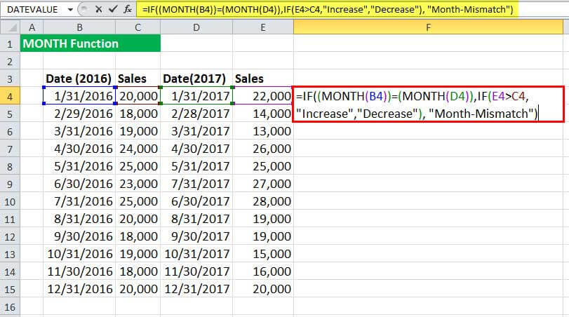
For the first entry, the MONTH function in Excel will return “Increase.”
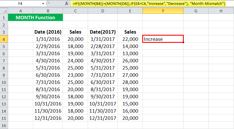
Let us look at the MONTH in Excel in detail:
If the MONTH of B4 (for 2016) is equal to the MONTH given in D4 (for 2017),
- The MONTH function in Excel will check if the sales for the given month in 2017 are greater than that in 2016.
- If it is greater, it will return “Increase.”
- Else, it will return to “Decrease.”
If the MONTH of B4 (for 2016) is not equal to the MONTH given in D4 (for 2017),
- The MONTH function in Excel will return “Mismatch.”
Similarly, you can do for the rest of the cells.
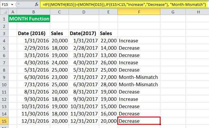
You could also add another condition to check if the sales are equal and return “Constant.”
MONTH in Excel Example #5
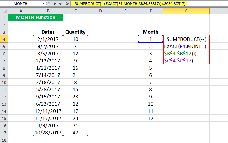
Suppose you work in your company's sales department and have date-wise data of how many products were sold on a particular date for the previous year, as shown below.
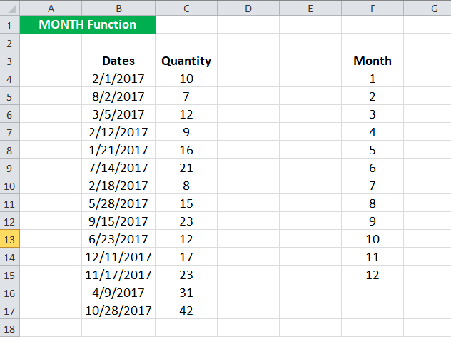
Now, you want to club the number of products monthly. To do so, you use the following MONTH formula in Excel:
= SUMPRODUCT(-- ( EXACT( F4, MONTH( $B$4:$B$17 ))), $C$4:$C$17 )
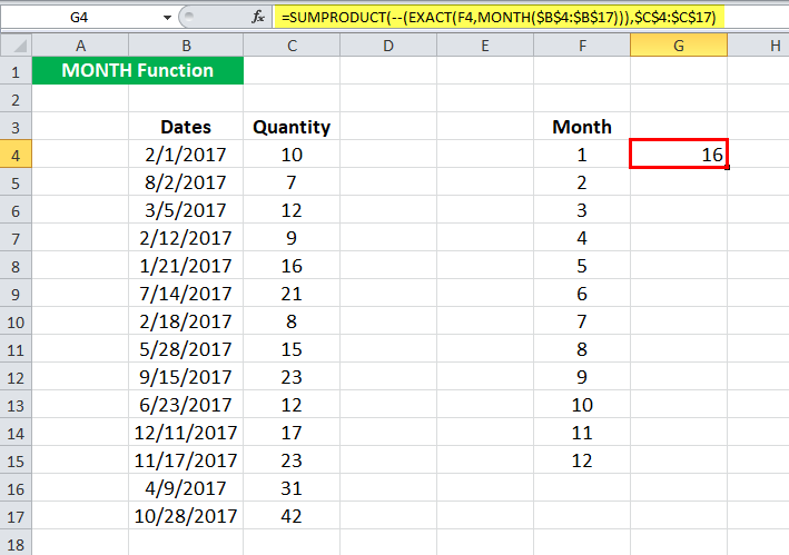
For the first cell, the MONTH function in Excel will return 16.
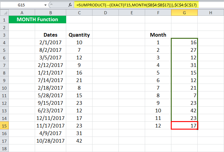
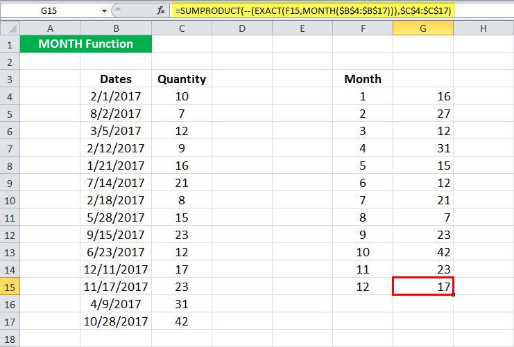
Then, drag it to the rest of the cells.
Let us look at the MONTH in Excel in detail:
= SUMPRODUCT(-- ( EXACT( F4, MONTH( $B$4:$B$17 ))), $C$4:$C$17 )
- MONTH( $B$4:$B$17 ) will give the month of the cells in B4: B17. MONTH function in Excel will return a matrix {2; 8; 3; 2; 1; 7; 2; 5; 9; 6; 12; 11; 4; 10}
- EXACT( F4, MONTH( $B$4:$B$17 )) will match the month in F4 ( 1 here) with the matrix and will return another matrix with TRUE when it is a match or FALSE otherwise. For the 1st month, it will return {FALSE; FALSE; FALSE; FALSE; TRUE; FALSE; FALSE; FALSE; FALSE; FALSE; FALSE; FALSE; FALSE; FALSE}
- SUMPRODUCT (– (..), $C$4:$C$17) will sum the values in C4:C17 when the corresponding value in the matrix is “TRUE.”
The MONTH function in Excel will return 16 for January.
Things to remember about a MONTH in Excel
- The MONTH function returns the month of the given date or serial number.
- Excel MONTH function is given #VALUE! Error when it cannot recognize the date.
- The Excel MONTH function accepts dates only after 1 Jan 1900. It will provide the #VALUE! Error when the input date is earlier than 1 Jan 1900.
- The MONTH function in Excel returns the month in number format only. Therefore, its output is always a number between 1 and 12.
