MINVERSE In Excel

Last Updated :

Blog Author :

Edited by :

Reviewed by :

Table Of Contents

What Is MINVERSE Function In Excel?

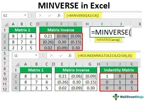
The MINVERSE function in Excel stands for "Matrix Inverse." This built-in Excel function converts the given matrix to the inverse matrix with the same number of arrays.

Having talked about the "inverse matrix," one needs to understand the "inverse matrix."

Inverse Matrix: The reciprocal of a number is called the "inverse matrix." For example, for the number 5, we can write the reciprocal as:

So, we can write the inverse matrix in the same logic using this equation "A-1." We can write the above number as 5-1 as well. When we multiply a number by its reciprocal we always get 1. For example, if the number 5 is multiplied by its reciprocal 1/5, we get the result of 13.

Similarly, when we multiply a matrix by its inverse, we get the identity matrix, "I." Below is the equation of the identity matrix.

A * A^-1 = I

When discussing the inverse matrix in Excel, we must look at the identity matrix. With an identity matrix, all the rows and columns are in equal numbers. So diagonally, we get 1 as the value; apart from diagonal, everything else will equal zero.

So, the identity matrix will always be "2 * 2, 3 * 3, 4 * 4" like this.

Once the matrix is inverted, we can cross-check whether it is inverted using the MMULT function in Excel. We will get an identity matrix that looks like this.

What Is MINVERSE Function In Excel?

The MINVERSE function in Excel converts a matrix to its inverse with the same number of arrays.
This function produces a #VALUE! Error when non-numeric values are included. It counts numbers and disregards empty cells, text, "TRUE" and "FALSE" logical values, and text values.
In the absence of numeric values in the input parameters, the function will return a zero as its output. It is important to note that the absence of numbers in the arguments will result in a 0 output.

Let us try these things with Excel now.

MINVERSE() Excel Formula

The MINVERSE function in Excel formula is

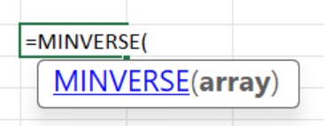
Where array is the only mandatory argument which denotes the range.

How To Use MINVERSE Excel Function?

Let us learn how to use MINVERSE Excel function with detailed examples.

Examples

Example #1 - Inverse Of The Matrix

For example, take a look at the below 3 * 3 matrix.

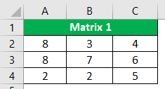
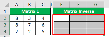
We have matrix numbers from A2 to C4. To reverse this matrix, create an identical table next to the above table but do not keep the same values and keep the field empty.

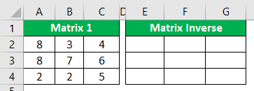
In the range E2 to G4, we will create an inverse of the matrix. First, select the range of cells from E2 to G4.

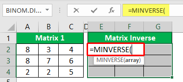
Now, in the selected range of cells, open the Excel MINVERSE function.

The first argument of the MINVERSE function is an array. It is the range of matrix values that we are trying to inverse, so our 3 * 3 matrix values are in the range of A2 to C4.

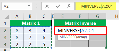
Before closing the formula, we need to remember that "MINVERSE" is an array, so we need to close out the formula using the "CSE" keys.

Note: CSE stands for “Ctrl + Shift + Enter”. So, all the array formulas are closed with these keys only.

So, close the formula by pressing the "ENTER" key by holding the "Ctrl + Shift" key together.

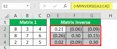
As we can see above, we have an "inverse matrix" using the MINVERSE function. Since it is an array formula, we can see curly brackets ({}) at the start and end of the array formula.

Example #2 - Using MMULT Function

We can cross-check whether this matrix is inversed or not by using the MMULT function. MMULT function stands for "Matrix Multiplication." Let us use the same data we used in Example 1.

Now, select the range of cells to create another identity matrix, so choose the 3 * 3 matrix area.

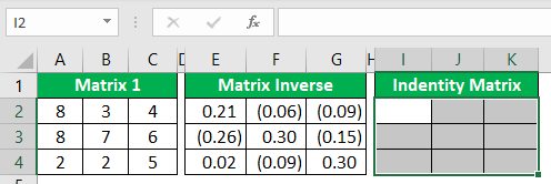
Now, open the MMULT function for the selected range of cells.

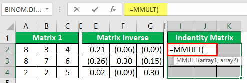
For the array1 argument of MMULT function, choose "Matrix 1" range from A2 to C4.

For the array2 argument of the MMULT function, choose the "inverse matrix" range of cells from E2 to G4.

The MMULT is also an array function, so close the formula by using the "CSE" keys to convert it to an array function.

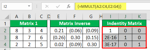
This result has given us decimal results, so use the ROUND function inside the array function to get an accurate "identity matrix."

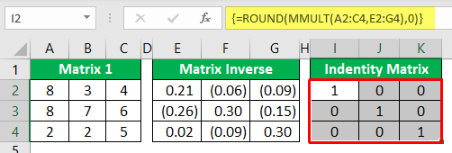
Now, we have an "identity matrix" with 1 as the diagonal value. Like this, we can use the MINVERSE function to inverse the matrix and MMULT to check whether it is reversed or not.

Example #3

Consider the below table.

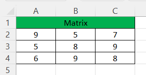
We have matrix numbers from A2 to C4.
Let us create an inverse matrix.
In the range E2 to G4, we will create an inverse of the matrix. First, select the range of cells from E2 to G4.

Now, in the selected range of cells, open the Excel MINVERSE function.

The first argument of the MINVERSE function is an array. It is the range of matrix values that we are trying to inverse, so our 3 * 3 matrix values are in the range of A2 to C4.

Before closing the formula, we need to remember that "MINVERSE" is an array, so we need to close out the formula using the "CSE" keys.

Note: CSE stands for “Ctrl + Shift + Enter”. So, all the array formulas are closed with these keys only.

So, close the formula by pressing the "ENTER" key by holding the "Ctrl + Shift" key together.

As we can see above, we have an "inverse matrix" using the MINVERSE function. Since it is an array formula, we can see curly brackets ({}) at the start and end of the array formula.

We can cross-check whether this matrix is inversed or not by using the MMULT function. MMULT function stands for "Matrix Multiplication." Let us use the same data we used in Example 1.

Now, select the range of cells to create another identity matrix, so choose the 3 * 3 matrix area.

Now, open the MMULT function for the selected range of cells.

For the array1 argument of MMULT function, choose "Matrix 1" range from A2 to C4.

For the array2 argument of the MMULT function, choose the "inverse matrix" range of cells from E2 to G4.

The MMULT is also an array function, so close the formula by using the "CSE" keys to convert it to an array function.

This result has given us decimal results, so use the ROUND function inside the array function to get an accurate "identity matrix."

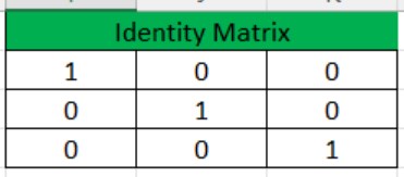
Now, we have an "identity matrix" with 1 as the diagonal value. Like this, we can use the MINVERSE function to inverse the matrix and MMULT to check whether it is reversed or not.

Important Things To Note

The MINVERSE function can accept only one matrix at a time.
It is an array function in Excel, so we must use the "CSE" keys to close the formula.
When the matrix is inverse, we can find the identity matrix using the MMULT function, where we need to multiply the original matrix with the inverse matrix.

Frequently Asked Questions

1. What is MINVERSE function error?

This error occurs when the provided array contains a blank or a non-numeric value or when it lacks equal numbers of rows and columns. The conditions above can lead to a mismatch in the dimensions of the array, and as such, the operation cannot be performed. It is essential to ensure that the array is of the correct data type and that it has uniform row and column numbers to avoid this error.

2. Why does MINVERSE not work in Excel?

If any cells in the array are empty or contain text, the MINVERSE function returns a #VALUE! Error. The MINVERSE function also returns a #VALUE! Error if the array does not have an equal number of rows and columns.

3. What is the meaning of MINVERSE?

The MINVERSE function produces an inverse matrix of an array that has an equal number of columns and rows. This mathematical tool is commonly employed in the resolution of systems of equations that involve multiple variables. The inversion of a matrix is a complex mathematical process that can be executed through the use of software applications, such as spreadsheet programs. Inverse matrices are critical in a wide range of fields, including engineering, finance, and physics, as they enable the optimization of solutions to complex mathematical problems.