Merge Tables In Excel

Last Updated :

Blog Author :

Edited by :

Reviewed by :

Table Of Contents

What Is Merge Tables In Excel?

When working in Excel, it is not definite that data will be in a single worksheet. It can be in multiple worksheets on multiple tables. If we want to merge tables, there are various methods to do that so that we can have data in a single table. It is known as merging tables in Excel. We can do this by using the VLOOKUP or INDEX and MATCH functions.

Consider the below image showing two tables in two different sheets.

However, we can see that column A is common in both sheets. In this case, we can merge tables such that the data is available in a single sheet.

Let us learn how to merge tables in Excel using detailed examples.

What Is Merge Tables In Excel?

Merge Tables in excel is used to merge or combine tables in Excel from multiple sheets.
It is used to compare and analyze data effectively.
Remember, to merge effectively, atleast one column should be common in the tables we want to merge.
The common column will work as the primary key while merging the tables from multiple sheets. Therefore, this is very important and should have unique values.
Using VLOOKUP, INDEX and MATCH functions, we can merge tables in Excel.

How To Merge 2 Tables In Excel?

As we already discussed, merging tables in excel is useful to analyze the data effectively. Now, let us learn how to merge tables in excel with the following examples.

Examples

Consider the below two tables.

Example #1 - Sheet 1: Table 1: BusinessInfo

We have given customer data city-wise in two tables. We have taken 20 records.

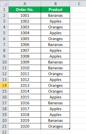
Example #2 - Sheet 2: Table 2: ProductDetails

Steps To Merge Tables In Excel

In both the tables, “Order No.” is the common information on which basis we will create a relationship between them.

Below are the steps for merging these two tables:

Click on any cell in the “Customer Info” table. Go to the “INSERT” tab and click on the “Table” option under the “Tables” section. You may refer to the below screenshot.
Then, the “Create Table” dialog box will appear. Our table “CustomerInfo” has column headers. Hence, the checkbox “My table has headers” should be checked. Refer to the below screenshot.
It will convert our data into a table format. Now, click on the “Table Name” field under the “Properties” section and give the name of this table as “Customer_Info.”

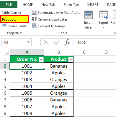
Follow the same steps for another table, “ProductDetails.” We have given the name “Products” to another table. Refer to the below screenshot.

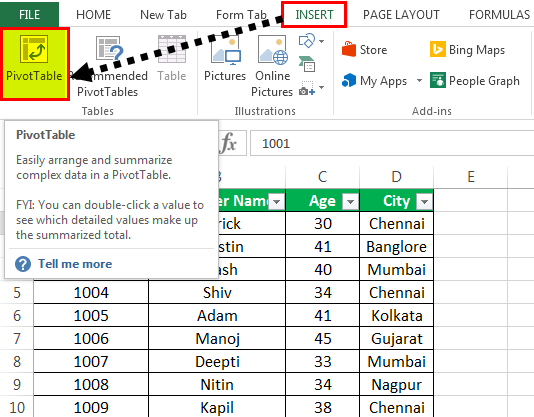
Click on somewhere on the “Customer_Info” table then, Then go to the “Insert” tab, and click on the “PivotTable” option under the “Tables” section.

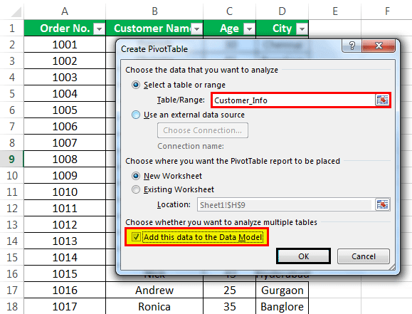
A dialog box for “Create PivotTable” will appear. Next, tick the checkbox “Add this data to the Data Model,” as shown in the below screenshot.

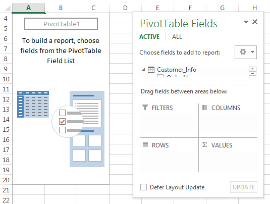
Click on "OK." Then, it will open a new sheet with a new Pivot Table Fields section on the right side, as shown in the below screenshot.

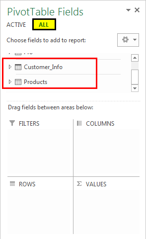
Click on the “ALL” tab in the “PivotTable Fields” section. It will display all the tables created by us. Refer to the below screenshot.

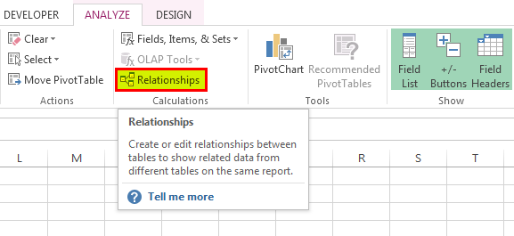
Now, click on the “Relationships” option under the “Calculations” section, as shown in the below screenshot.

It will open a dialog box for creating a relationship between these tables. First, click on the “New” button. Then, refer to the below screenshot.

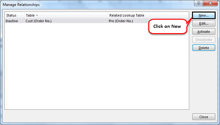
Again, it will open a dialog box as shown below, and created tables are listed here.

As there is one field, “Order No.” is common in both tables. Hence we will create a relationship between these tables using this common field/column.
Select “Customer_Info” under the “Table” section and the “Order No.” field under the “Column (Foreign)” section. Then, refer to the below screenshot.

Select another table, “Products,” under the “Related Table” section and select the “Order No.” field under the “Related Column” section. Then, refer to the below screenshot.

The primary key is the unique values that appear once in the table. Then, click on “OK.” It will display the relationship, as shown in the below screenshot.

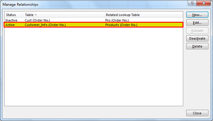
Now, we can drag and drop the field accordingly to see the result. Next, click on the “Customer_Info” table, as shown in the below screenshot.

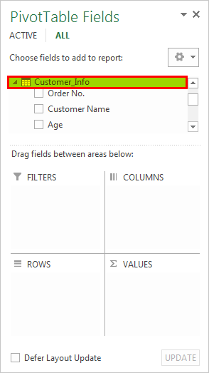
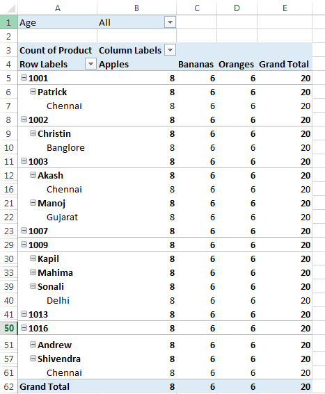
Under the “ROWS” box, drag fields “Order No.”, “Customer Name,” and the “City.”
Drag the “Age” field under the “FILTERS” box.
Drag the “Product” field under the “COLUMNS” box, and the “VALUES” box for the products count.

The final result is below:

Accordingly, as per the requirement, we can drag and drop the fields.

Important Things To Note

As the name suggests, merge tables in excel is used to merge tables in excel from multiple sheets.
We can merge more than two tables using this process.
There should be one column common in each table.
There are many ways to merge the data from multiple tables into one table in excel

Frequently Asked Questions

1. What is merge tables in excel?

Merge tables in excel, as its name, helps users merge tables from different sheets in Excel. We can use VLOOKUP, Index and Match functions to merge tables in Excel.

2. How can we merge tables in excel?

Merging tables in Excel is simple.
Consider the below image showing two tables in two different sheets.

FAQ 2

However, we can see that column A is common in both sheets. In this case, we can merge tables such that the data is available in a single sheet.

Now, this common table will be the connection and using any of the mentioned methods, we can merge tables in excel.

3. What is the difference between merge cells and merge tables?

Merge cells is used to merge cells to enhance the presentation of our data in worksheet. But, merge tables in excel is used to combine two different tables to compare and analyze data effectively.