Linear Interpolation In Excel

Linear interpolation in Excel means forecasting or guessing the next value of any certain variable given on the current data. Here, we create a straight line that connects two values and estimates the future value. In Excel, we use a FORECAST function and a LOOKUP function to do a linear interpolation.

Interpolation is a mathematical or statistical tool that predicts the values between two points on a curve or line. We can use this tool in statistics and other fields like business, science, etc., wherever there is an opportunity to predict values between two data points.

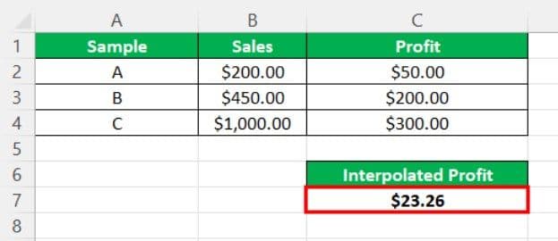
For example, consider the below image showing the sales and profit of various products.

Now, we can find the linear interpolation in Excel using FORECAST formula.

The result will appear as shown in the below image.

Likewise, we can use linear interpolation in Excel.

• Linear interpolation in Excel refers to predicting the next variable value based on present data. It involves making a straight line connecting two known values and using the same to predict future values. One can use either the FORECAST function or the LOOKUP function.
• Despite being the least accurate method, it is a quick method for making precise estimates when table values are closely spaced. Also, it is helpful in estimating geographical data points, rainfall, noise levels, and similar applications. 
• It is easy but needs improvement in accuracy for nonlinear functions. Polynomial and spline are other Excel interpolation methods.

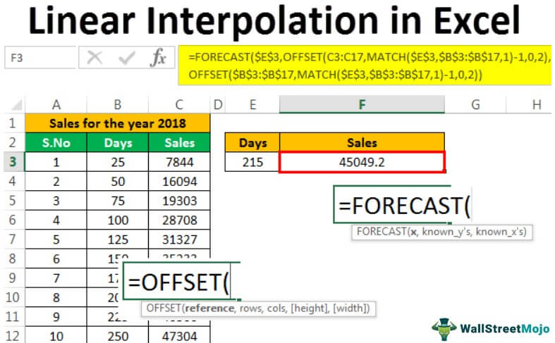
We can calculate linear interpolation in Excel using FORECAST in Excel.

The function is =FORECAST(x,known_ys,known_xs)

Where,

• x: The data point for which you require to estimate the value.
• known_ys: The dependent data range.
• known_xs: The independent data range.

Note that all 3 arguments are mandatory.

We have to use a few formulas in Excel like FORECAST, OFFSET, and MATCH. Let us see in brief these formulas before we go ahead.

FORECAST

FORECAST() – This Forecast excel function calculates or predicts the future value based on existing values and a linear trend.

• X – This is the value for which we want to predict.
• Known_ys – This is the dependent value from the data and a mandatory field to be filled
• Known_xs – This is the independent value from the data and a required field to be served.

MATCH

MATCH() – This Match excel function will return the relative position of a lookup value in a row, column, or table that matches the specified value in a specified order.

• Lookup_value – This is the value that needs to be matched from the lookup_array
• Lookup_array – This is the range for searching

– This can be 1,0,-1. The default would be 1. For the 1 – MATCH function, you will find the largest value less than or equal to the look_up value. The value should be in ascending order. For 0 – MATCH function finds the first value exactly equal to lookup_value and no need to be sorted. For -1 – Match will find the smallest value greater than or equal to the look_up value and should be sorted in descending order.

OFFSET

OFFSET() – This Offset function will return a cell or range of cells which are specified number of rows and columns. The cell or range of cells will depend on the height and width of rows and columns we specify.

• Reference – This is the starting point from where it will count rows and columns will be done.
• Rows – Number of rows to offset below the starting reference cell.
• Columns - Number of columns to offset right from the starting reference cell.
• – The height in rows from the returned reference. It is optional.
• – The width in columns from the returned reference. It is optional.

Example #1

Performing Interpolation to know the temperature of weather during different time zones

First, take down the temperature figures of the Bangalore region for each hour, and the data would be as follows: –

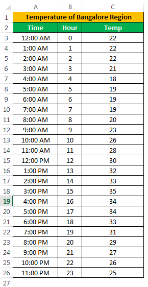
The data shows that we have got the temperature details of the Bangalore region for some date. We have the time zones for the entire day in the on-time column. In the hour column, we mention the hours from the start of the day, like 12:00 AM would be 0 hours, 1:00 AM would be 1 hour, and so on.

We will perform interpolation for the data to pull out the temperature value for the required time zone, which may be any time, not only the exact hour.

Type the formula in a cell that we need to see the temperature for different time zone. It tells that we have to select the cell that needs to be forecasted, and the OFFSET and MATCH function is used to determine the known_ys and known_xs.

FORECAST($F$5 – Select the cell that has the time zone to be forecasted.

OFFSET($C$3:$C$26,MATCH($F$5,$B$3:$B$26,1)-1,0,2) – This is used to select the known_ys as a reference is taken temp column because these are the dependent values. The match function is used to generate the position of the value that we need to forecast and calculate the number of rows. Columns should be 0 because we want the dependent value on the same column selected and height to be 2 as we need to perform the forecast based on the last two values.

OFFSET($B$3:$B$26, MATCH($F$5,$B$3:$B$26,1)-1,0,2) – This is used to select the known_xs as a reference is taken hour column because these are independent values and rest is the same as we had done for row count.

Now give some time zone in the cell that we had considered forecasting. Here, the value entered is 19.5, which is 7:30 PM, and we will get the temperature of 30, which is forecasted from the temperature values given on an hourly basis.

Similarly, this formula can show temp figures for different time zones.

Example #2

Performing Linear Interpolation to know the sales of an organization in 2018

Let us assume that we got the sales details for an organization in 2018 as below.

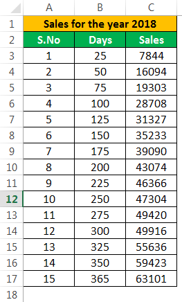
We can use the same formula we used in interpolation to forecast sales value for different days, which we did not mention in the data we considered. Here the sales are in a straight line(linear) as we had taken cumulatively.

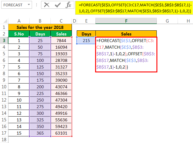
If we want to see the number of sales we had achieved in 215 days, we can get the forecasted number of sales for 215 days as below by considering the given sales data.

Similarly, we can determine the number of sales in that year by forecasting between the given points.

Example #3

For example, consider the below image showing the sales and profit of various products.

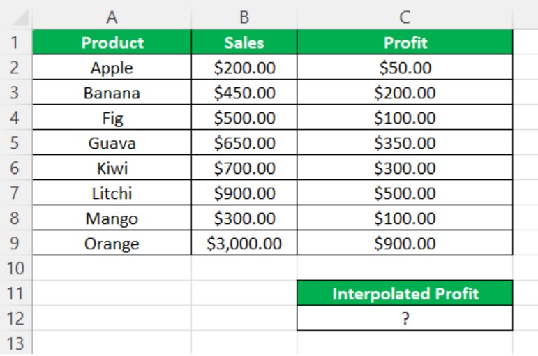
Now, we can find the linear interpolation in Excel using FORECAST formula.

So, the formula is =FORECAST(B12,C2:C9,B2:B9).

The result will appear as shown in the below image.

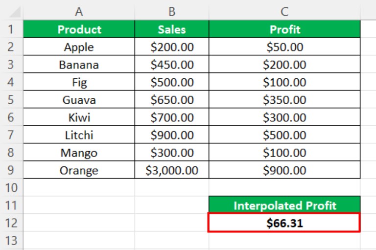
Likewise, we can use linear interpolation in Excel.

• This method is fast and precise when the table values are closely spaced. But remember that the method is least accurate.
• We can use the method to estimate values for geographical data points, rainfall, noise levels, etc.
• It is very easy to use and not very accurate for nonlinear functions.
• Apart from Excel linear interpolation, we also have different methods like polynomial interpolation, spline interpolation, etc.

This article is a guide to Linear Interpolation in Excel. Here, we will see how to perform interpolation and linear interpolation in Excel, some examples, and a downloadable Excel template. You may learn more about Excel from the following articles: -

• Formula of Relative Change
• Complete list of Excel Functions
• Formula for Standard Normal Distribution