LEFT Function in Excel

The LEFT formula in Excel accepts the following parameters and arguments:

text- Required. It is referred to as the string that you wish to extract from.

number_of_characters – . It is referred to as the number of characters you want to extract, starting from the leftmost character. Note that if this parameter is omitted, it will return only 1 character.

Return Value:

The return value will be either a string or a text value.

• We should use the LEFT function in Excel for extracting characters starting from the left side of the text.
• Number_of_characters is optional and defaults to 1.
• The LEFT function in Excel will extract digits from numbers as well.
• Number formatting (the currency symbol $) is not part of a number. Therefore these are not counted or extracted by the EXCEL LEFT function.

Below are some of the examples of LEFT functions in Excel.

1. We can insert the desired LEFT formula in Excel in the required cell to attain a return value on the argument.
2. We can manually open the LEFT formula in the Excel dialog box in the spreadsheet and enter the text and number of characters.

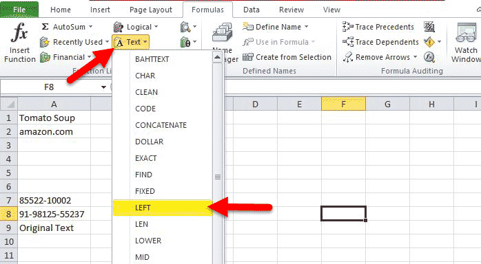
3. We can see the LEFT formula in the Excel option under the "Text" tab of the "Formulas" tab in the menu bar from the above spreadsheet.
4. To open the LEFT formula in the Excel dialog box, click on the "Text" tab under the "Formulas" tab and click "LEFT." See the sample below.

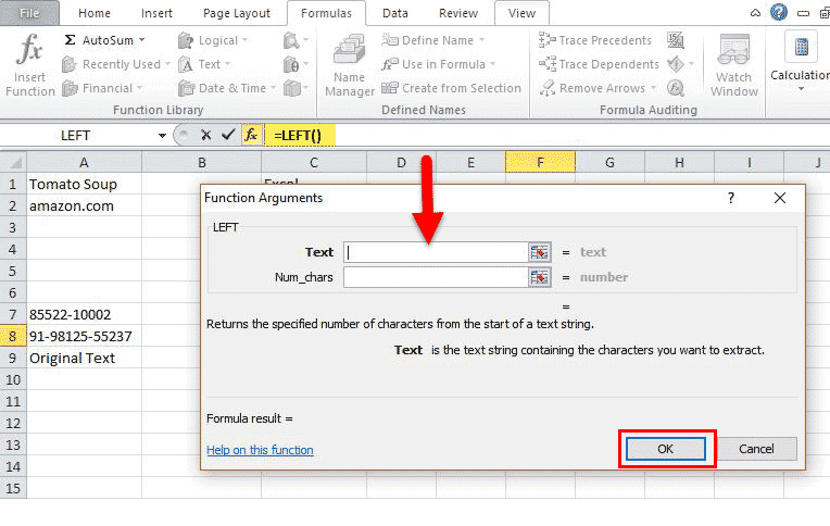
5. The above dialogue box will open where you can put the arguments to attain a “Formula result.”

Extracting a substring before a certain character:

We can use the below given generic formula for getting a substring that precedes any other character:

The above LEFT formula in Excel is used when we want to extract the part of the text string which is preceding a specific character. For example, if we are going to pull the first names from a column of full names or we want to extract the country codes from the list of phone numbers.

Removing the last N characters from a string:

You can use the following generic formula for removing the last N characters from a string.

The above LEFT formula in Excel is used when we want to remove a certain number of characters from the end of the string and pull the rest of the string into another cell. The working of the LEFT formula in Excel is based on the logic: the LEN function is used to get the total number of characters in a string. The LEFT formula in Excel subtracts the number of unwanted characters from the total length, and the LEFT function in Excel returns the remaining characters.

1. Worksheet Function

Let us look below at some examples of the LEFT function in Excel. These examples will help you explore the use of the LEFT function in Excel.

In the above spreadsheet, the LEFT formula in excel written is =LEFT (A1, 5).

The result based on the syntax of the LEFT function is TOMAT.

Let’s look at some more examples –

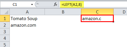
When the LEFT formula in Excel is written is =LEFT (A2, 8)

Result: amazon.c

Consider the Excel spreadsheet below.

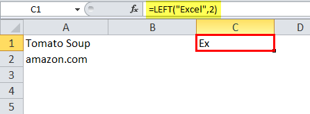
When the LEFT formula in Excel is written, as =LEFT (“Excel”, 2)

Result: “Ex”

Consider the Excel spreadsheet below.

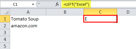
When the LEFT formula is written as = LEFT (“EXCEL”)

Result: “E”

Consider the Excel spreadsheet below

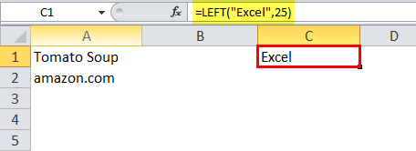
When the LEFT formula is written, as =LEFT (“Excel”, 25)

Result: “Excel”

Look at the spreadsheet below to understand the above example.

Consider the data below, which is put in an Excel spreadsheet.

• 85522-10002
• 91-98125-55237
• Original Text

These are the return values for the Excel LEFT function mentioned.

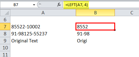
• When the LEFT formula in Excel is entered as =LEFT(A7,4), the result is 8552.
• When the LEFT formula in Excel is entered as =LEFT(A8,5), the result is 91-98.
• When the LEFT formula in Excel is entered as =LEFT(A9,5), the result is Origi.

2. LEFT Function VBA

You can also use the LEFT function VBA Code in Microsoft Excel.

Look at the below examples to understand the LEFT function as a VBA function.

Extracting a substring of length 4 from the start of the string Kelly Michael.

The variable res is now equal to the text string Kell.

In the above example, the LEFT function VBA returns the result, Kell.

Extracting a substring of length 8 from the start of the string Kelly John Michael.

The variable res will now equal the text string “Kelly Joh.”

In the above example, VBA LEFT function returns the result “Kelly Joh.”

• The LEFT in Excel is a function by which we can extract a substring from a string, starting from the leftmost character.
• The return value can be a string or text value.
• The return value depends on the arguments we input in the formula syntax of the OR function.
• #VALUE! Error – This occurs if the given (number_of_characters) argument is less than 0.
• Dates are put away in Excel as numbers, and it is just the cell formatting that makes them show up as dates in our spreadsheet. Therefore, if we attempt to use the Excel LEFT function on a date, it will return the number's starting characters that represent that date.